library(ggplot2)

theme_te <- function() {
  theme_minimal(base_size = 12) +
    theme(plot.background  = element_rect(fill = "#f5f4ee", colour = NA),
          panel.background = element_rect(fill = "#f5f4ee", colour = NA),
          panel.grid.minor = element_blank(),
          panel.grid.major = element_line(colour = "#dad9ca", linewidth = 0.3),
          plot.title    = element_text(colour = "#16241d", face = "bold", size = 12),
          plot.subtitle = element_text(colour = "#5d6b61", size = 9.5),
          axis.title    = element_text(colour = "#46604a", size = 10),
          axis.text     = element_text(colour = "#2c3a31", size = 9),
          legend.text   = element_text(colour = "#2c3a31", size = 9),
          legend.title  = element_text(colour = "#46604a", size = 9.5))
}Beta diversity as variance: LCBD and SCBD
R
beta diversity
LCBD
biodiversity
ecology tutorial
Computing BD, LCBD and SCBD from scratch in base R, with the exact sum-of-squares identity, the bound nobody quotes, and two measured traps in how LCBD is read.
Corrected 15 October 2026: the heading of the first trap stated that the poorest site wins, as if that were the rule, when poverty puts a site near the top and its particular species decide first place; it now says that poor sites rank high.
Corrected 7 October 2026: the post called beta diversity as a variance the same arithmetic as an average pairwise dissimilarity, when it equals half the average squared pairwise dissimilarity; and it said the poorest site took the top LCBD spot for having six species and that the rarest-species control settled this, when poverty puts that site near the top and the particular six species it drew decide first place.
Corrected 30 September 2026: the richness control said that the unchanged rank showed species identity contributed nothing; the site was already ranked first, so its rank could not rise, and the text now says its LCBD rises only modestly when its species become the rarest.
Every beta diversity measure so far in this series returns one number for the whole dataset. That number cannot be mapped. It cannot rank sites for protection. It cannot tell you which species drives the pattern.
Legendre and De Caceres (2013) took a different route: treat the site-by-species table as data, and let beta diversity be its total variance. The move sounds like bookkeeping. It is not, because a variance decomposes: into rows, giving you a number per site, and into columns, giving you a number per species. That is where LCBD and SCBD come from, and it is why the framing spread so fast into conservation work.
It also comes with two failure modes that are easy to measure and easy to miss.
Setup
The quantity
Take the community table, transform it, centre each column, and add up the squares. That total sum of squares is the beta diversity. Divide by n - 1 and it is a variance:
hellinger <- function(Y) sqrt(Y / rowSums(Y))

beta_div <- function(Y, transform = hellinger) {
  Z  <- transform(Y)
  C  <- sweep(Z, 2, colMeans(Z))        # centre each species column
  SS <- sum(C^2)
  list(SS      = SS,
       BDtotal = SS / (nrow(Y) - 1),
       LCBD    = rowSums(C^2) / SS,     # each site's share of the variance
       SCBD    = colSums(C^2) / SS)     # each species' share
}
That is the whole method. Nine lines, no package.
The identity that makes it work
The definition above needs a transformation and a centring. But the same sum of squares can be read off a dissimilarity matrix, with no centring anywhere, through a Gower-centred distance matrix. The two routes agree exactly, and that agreement is what lets the method accept any dissimilarity coefficient you like:
set.seed(306)
Y <- matrix(rpois(15 * 40, 4), 15, 40)
Y[cbind(sample(15, 60, TRUE), sample(40, 60, TRUE))] <- 0    # some zeros, as usual

d_hell <- as.matrix(dist(hellinger(Y)))

gower_trace <- function(D) {                       # SS straight from a dissimilarity matrix
  A <- -0.5 * D^2
  G <- sweep(sweep(A, 1, rowMeans(A)), 2, colMeans(A)) + mean(A)
  sum(diag(G))
}

bd <- beta_div(Y)
c(SS_from_centring  = bd$SS,
  SS_from_distances = gower_trace(d_hell),
  SS_from_pairs     = sum(d_hell[upper.tri(d_hell)]^2) / nrow(Y),
  gap = max(abs(c(gower_trace(d_hell), sum(d_hell[upper.tri(d_hell)]^2) / nrow(Y)) - bd$SS)))
SS_from_centring SS_from_distances SS_from_pairs gap
2.357883e+00 2.357883e+00 2.357883e+00 1.332268e-15 Three routes, one number. The third is the most useful one to remember: the sum of squares is the sum of squared pairwise distances divided by the number of sites. Beta diversity as a variance and beta diversity as half the average squared pairwise dissimilarity are the same arithmetic, seen from two sides.
The shares behave as shares should:
c(sum_LCBD = sum(bd$LCBD), sum_SCBD = sum(bd$SCBD),
  n_sites = nrow(Y), expected_LCBD_if_uniform = 1 / nrow(Y))
sum_LCBD sum_SCBD n_sites
1.00000000 1.00000000 15.00000000
expected_LCBD_if_uniform
0.06666667 Any coefficient, including the awkward ones
Because the distance route needs no centring, you can feed it Bray-Curtis, which is not a Euclidean distance. On a table holding sites that share no species at all, the Gower-centred matrix has a negative eigenvalue, which would break a principal coordinates analysis. It does not break the trace:
bray <- function(Y) {
  n <- nrow(Y); D <- matrix(0, n, n)
  for (i in 1:n) for (j in 1:n)
    D[i, j] <- sum(abs(Y[i, ] - Y[j, ])) / sum(Y[i, ] + Y[j, ])
  D
}

Ys <- Y
Ys[1:5, 21:40] <- 0        # five sites hold only the first half of the pool
Ys[6:10, 1:20] <- 0        # five hold only the second half, so the blocks share nothing

d_bray <- bray(Ys)
A <- -0.5 * d_bray^2
G <- sweep(sweep(A, 1, rowMeans(A)), 2, colMeans(A)) + mean(A)
ev <- eigen(G, symmetric = TRUE, only.values = TRUE)$values

c(smallest_eigenvalue = min(ev),
  is_euclidean        = min(ev) > -1e-8,
  SS_from_trace       = sum(diag(G)),
  SS_from_pairs       = sum(d_bray[upper.tri(d_bray)]^2) / nrow(Ys),
  gap = abs(sum(diag(G)) - sum(d_bray[upper.tri(d_bray)]^2) / nrow(Ys)))
smallest_eigenvalue is_euclidean SS_from_trace SS_from_pairs
-4.531939e-02 0.000000e+00 3.020802e+00 3.020802e+00
gap
8.881784e-16 The smallest eigenvalue is negative, so the Bray-Curtis matrix is not embeddable in Euclidean space, and the two sum-of-squares routes still agree to within floating-point rounding (the gap entry printed above). The trace is a sum of squared distances to the centroid, and that quantity does not care whether the space is Euclidean.
What BD is bounded by
BD has a maximum, and it is not what people expect. Put n sites together with no species shared between any of them, so the data is as beta-diverse as data can be, and vary everything else:
max_tab <- do.call(rbind, lapply(c(2, 5, 20), function(n) {
  do.call(rbind, lapply(c(3, 25), function(S) {
    Yd <- matrix(0, n, n * S)
    for (i in 1:n) Yd[i, ((i - 1) * S + 1):(i * S)] <- rpois(S, 10) + 1
    jac <- as.matrix(dist(Yd > 0, method = "binary"))
    data.frame(n_sites = n, species_per_site = S,
               BD_jaccard   = gower_trace(jac) / (n - 1),
               BD_hellinger = beta_div(Yd)$BDtotal)
  }))
}))
knitr::kable(max_tab, digits = 10,
col.names = c("sites", "species per site", "BD with Jaccard", "BD with Hellinger"))| sites | species per site | BD with Jaccard | BD with Hellinger |
|---|---|---|---|
| 2 | 3 | 0.5 | 1 |
| 2 | 25 | 0.5 | 1 |
| 5 | 3 | 0.5 | 1 |
| 5 | 25 | 0.5 | 1 |
| 20 | 3 | 0.5 | 1 |
| 20 | 25 | 0.5 | 1 |
Exactly 0.5 for Jaccard and exactly 1 for Hellinger, whatever the number of sites, whatever the richness. The reason is one line of algebra: with all pairwise distances at their maximum Dmax, the sum of squares is (n-1)/2 * Dmax^2, so BD is Dmax^2 / 2. Jaccard caps at 1, so BD caps at 0.5. Hellinger caps at the square root of 2, so BD caps at 1.
Which means a BD of 0.3 is 60% of the way to maximal turnover under Jaccard, and 30% of the way under Hellinger. BD values from different coefficients are not comparable, and neither are BD values quoted without their coefficient. Legendre and De Caceres (2013) state the bound; it disappears from most of the papers that use the method.
Trap one: poor sites rank high
LCBD is sold as ecological uniqueness, and uniqueness sounds like a good thing to conserve. Build a dataset where the answer is known and look.
The design below is deliberately stripped: thirty sites, one shared species pool, one shared abundance profile. No environmental gradient. No site has a species another site could not have. The only thing that differs between sites is how many species each one drew.
set.seed(3064)
n <- 30; S <- 60
pool <- rlnorm(S, 0, 0.8)                          # one pool, one abundance profile, shared by all
k_of <- round(seq(6, 55, length.out = n))          # the only thing that varies: species count

Yg <- t(sapply(seq_len(n), function(i) {
  y  <- numeric(S)
  sp <- sample(S, k_of[i], prob = pool)
  v  <- rpois(k_of[i], 40 * pool[sp] / mean(pool)); v[v == 0] <- 1
  y[sp] <- v
  y
}))

bg   <- beta_div(Yg)
rich <- rowSums(Yg > 0)

c(spearman_LCBD_richness = cor(bg$LCBD, rich, method = "spearman"),
  richness_of_poorest = min(rich), LCBD_rank_of_poorest = rank(-bg$LCBD)[which.min(rich)],
  richness_of_richest = max(rich), LCBD_rank_of_richest = rank(-bg$LCBD)[which.max(rich)],
  LCBD_of_poorest = bg$LCBD[which.min(rich)], LCBD_if_uniform = 1 / n)
spearman_LCBD_richness richness_of_poorest LCBD_rank_of_poorest
-0.98442714 6.00000000 1.00000000
richness_of_richest LCBD_rank_of_richest LCBD_of_poorest
55.00000000 30.00000000 0.12174272
LCBD_if_uniform
0.03333333 The correlation between LCBD and richness is -0.98. The site with 6 species ranks 1 out of 30 for ecological uniqueness, holding 3.7 times its equal share of the variance. The site with 55 species ranks last.
Now a control. Give that poorest site the six rarest species in the pool, which is the situation everyone pictures when they read “high LCBD”:
Yr <- Yg
Yr[which.min(rich), ] <- 0
Yr[which.min(rich), order(pool)[1:6]] <- 30       # same site, same count, now the rarest species

c(rank_with_ordinary_species = rank(-bg$LCBD)[which.min(rich)],
  rank_with_rarest_species   = rank(-beta_div(Yr)$LCBD)[which.min(rich)],
  n_sites = n)
rank_with_ordinary_species rank_with_rarest_species
1 1
n_sites
30 The rank does not move, but it could not have risen: the site was already first. Making its six species the rarest in the pool raises its LCBD only modestly, partly because the six species it drew were, as a set, already unusually uncommon for a draw from this pool. With a more typical draw of six species the site would still rank near the top, but usually not first: poverty puts it high, and which six species it holds decides the top spot.
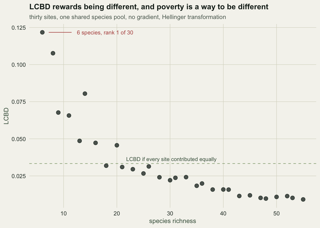
There is no bug here. LCBD measures squared distance from the average composition, and a site with six species is very far from the average composition. Whether that makes it valuable is an ecological judgement the arithmetic cannot make for you. Legendre and De Caceres (2013) are explicit that a high LCBD can indicate degradation as easily as it indicates rarity; the field mostly reads it the other way.
The practical move: never publish an LCBD map without the richness map beside it, and check the correlation between them before you interpret a single site.
Trap two: the coefficient picks the winner
Take one site and change nothing about its species list. Only redistribute its abundances so that one species dominates completely:
set.seed(3062)
Yc <- matrix(rpois(20 * 30, 6), 20, 30)                 # zeros happen, so species lists differ
Yc[cbind(sample(20, 90, TRUE), sample(30, 90, TRUE))] <- 0
Yc[rowSums(Yc) == 0, 1] <- 1
present13 <- which(Yc[13, ] > 0)                        # site 13 keeps its species list exactly
Yc[13, present13] <- 1
Yc[13, present13[1]] <- 400                             # and lets one of them take over completely

lcbd_hell <- beta_div(Yc)$LCBD
jac_d     <- as.matrix(dist(Yc > 0, method = "binary"))
Aj <- -0.5 * jac_d^2
Gj <- sweep(sweep(Aj, 1, rowMeans(Aj)), 2, colMeans(Aj)) + mean(Aj)
lcbd_jac <- diag(Gj) / sum(diag(Gj))

c(site13_species_count = sum(Yc[13, ] > 0),
  site13_share_of_top_species = max(Yc[13, ]) / sum(Yc[13, ]),
  site13_rank_hellinger = rank(-lcbd_hell)[13],
  site13_rank_jaccard   = rank(-lcbd_jac)[13],
  spearman_between_the_two = cor(lcbd_hell, lcbd_jac, method = "spearman"),
  BD_hellinger = beta_div(Yc)$BDtotal,
  BD_jaccard   = sum(diag(Gj)) / (nrow(Yc) - 1))
site13_species_count site13_share_of_top_species
26.00000000 0.94117647
site13_rank_hellinger site13_rank_jaccard.13
1.00000000 14.00000000
spearman_between_the_two BD_hellinger
0.80000000 0.22738341
BD_jaccard
0.03357418 Site 13 keeps all 26 of its species and gives 94% of its individuals to one of them. It ranks 1 of 20 under Hellinger and 14 of 20 under Jaccard. The rank correlation between the two LCBD vectors is 0.80. Jaccard cannot see the change at all, because Jaccard reads presence and absence, and site 13 did not lose a single species.
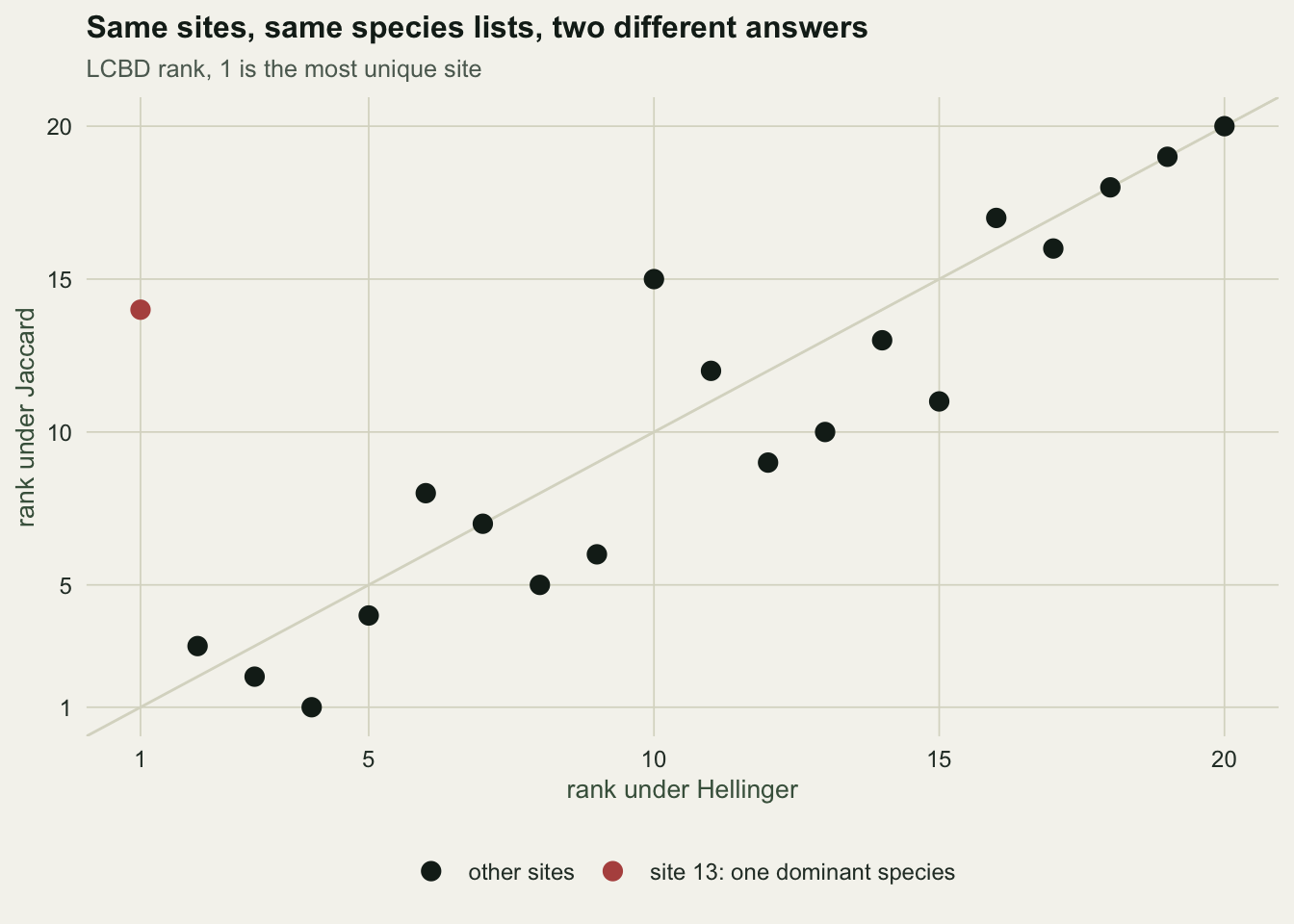
If your question is about composition in the presence-absence sense, Jaccard is the right answer and Hellinger is over-reading noise. If your question is about community structure, the reverse. The coefficient is not a technical detail to be defaulted; it is the ecological question, written in matrix form. Legendre and Gallagher (2001) is the reference for choosing among the transformations, and it is worth reading before you pick one.
Testing an LCBD
A high LCBD is not evidence of anything until you know what a high LCBD looks like under a null. The test in Legendre and De Caceres (2013) permutes within columns, which preserves each species’ abundance distribution while destroying the association between species at a site:
lcbd_test <- function(Y, nperm = 999) {
  obs <- beta_div(Y)$LCBD
  cnt <- rep(1, length(obs))                        # the observed value counts as one
  for (k in 1:nperm) {
    Yp <- apply(Y, 2, sample)                       # permute each species column independently
    cnt <- cnt + (beta_div(Yp)$LCBD >= obs)
  }
  cnt / (nperm + 1)
}

set.seed(3063)
pvals <- lcbd_test(Yg, nperm = 499)
signif_sites <- which(pvals <= 0.05)

data.frame(site = signif_sites, richness = rich[signif_sites],
           LCBD = round(bg$LCBD[signif_sites], 4), p = pvals[signif_sites])
site richness LCBD p
1 1 6 0.1217 0.002
2 2 8 0.1077 0.002
3 3 9 0.0677 0.012
4 4 11 0.0657 0.004
5 6 14 0.0804 0.0025 of 30 sites clear the 0.05 line, with p values down to 0.002. Look at their richness column: they are 5 of the six poorest sites in the dataset, and the dataset has no ecological structure in it at all.
That is the part worth sitting with. The permutation test is doing its job correctly. It asks whether a site’s composition is more distinctive than a reshuffle of the same species pool, and for a six-species site the answer is a confident yes. Significance does not protect you from the trap above; it certifies the trap with a small p value. A significant LCBD means “this composition is unlikely under column-wise reshuffling”, which is a much narrower claim than “this site is ecologically special”, and no amount of permutation closes the gap between the two.
Honest limits
LCBD is a share, so it depends on n. Every LCBD sums to 1, so the average is always 1/n. An LCBD of 0.10 is enormous in a 30-site study and unremarkable in a 5-site one. Report n, or report LCBD as a multiple of 1/n.
The site set defines the answer. LCBD measures distance from the average of your sites. Add a new habitat and every existing LCBD changes, because the average moved. This is not noise, it is the definition, and it means LCBD is not a property of a site that you can carry between studies.
BD is not comparable across coefficients. See the maximum above: the same data gives 0.5 with Jaccard and 1.0 with Hellinger at full turnover.
Zeros are not an ecological signal. The transformation is doing a lot of work here. A raw Euclidean distance on untransformed abundances treats two sites as similar for sharing absences, which is why the Hellinger and chord transformations exist in the first place.
Where to go next
The variance framing and the multiplicative framing answer different questions and can disagree about the same data. If you want the effective-number version, that is multiplicative beta diversity. If you want to know which sites share species with which others, zeta diversity is the multi-site view. And if you want to decompose the dissimilarity into turnover and nestedness rather than into sites, that is beta diversity partitioning; Legendre (2014) discusses a different split, into replacement and richness difference.
The most useful habit: compute BD twice, with two coefficients, before writing anything about which sites matter. If the rankings agree, say so. If they do not, you have learned something about your data that one number would have hidden.
References
Legendre & De Caceres 2013 Ecology Letters 16(8):951-963 (10.1111/ele.12141)
Legendre & Gallagher 2001 Oecologia 129(2):271-280 (10.1007/s004420100716)
Legendre 2014 Global Ecology and Biogeography 23(11):1324-1334 (10.1111/geb.12207)