library(ggplot2)

theme_te <- function() {
  theme_minimal(base_size = 12) +
    theme(plot.background  = element_rect(fill = "#f5f4ee", colour = NA),
          panel.background = element_rect(fill = "#f5f4ee", colour = NA),
          panel.grid.minor = element_blank(),
          panel.grid.major = element_line(colour = "#dad9ca", linewidth = 0.3),
          plot.title    = element_text(colour = "#16241d", face = "bold", size = 12),
          plot.subtitle = element_text(colour = "#5d6b61", size = 9.5),
          axis.title    = element_text(colour = "#46604a", size = 10),
          axis.text     = element_text(colour = "#2c3a31", size = 9),
          legend.text   = element_text(colour = "#2c3a31", size = 9),
          legend.title  = element_text(colour = "#46604a", size = 9.5))
}

hill <- function(p, q) {
  p <- p[p > 0]
  if (abs(q - 1) < 1e-10) return(exp(-sum(p * log(p))))
  sum(p^q)^(1 / (1 - q))
}
alpha_jost <- function(Y, q) {
  P <- Y / rowSums(Y)
  if (abs(q - 1) < 1e-10)
    return(exp(mean(apply(P, 1, function(p) { p <- p[p > 0]; -sum(p * log(p)) }))))
  mean(apply(P, 1, function(p) { p <- p[p > 0]; sum(p^q) }))^(1 / (1 - q))
}
beta_mult <- function(Y, q) hill(colMeans(Y / rowSums(Y)), q) / alpha_jost(Y, q)

good_turing <- function(x) {                       # sample coverage of the sample you have
  n <- sum(x); f1 <- sum(x == 1); f2 <- sum(x == 2)
  if (f1 == 0) return(1)
  1 - (f1 / n) * ((n - 1) * f1 / ((n - 1) * f1 + 2 * f2))
}Checking a beta diversity analysis
R
beta diversity
biodiversity
model checking
ecology tutorial
Three checks to run before interpreting a beta diversity result: sampling effort, the choice of metric, and the site set. Each one can flip the verdict.
Corrected 8 October 2026: the site-set check explained the fall in BD by the larger denominator alone; it now says that the new sites added less than their share to the sum of squares. The metric figure drew each multiplicative beta from zero, so a region with no turnover still showed a sizeable bar, and now draws the excess over one; and the report list no longer says that LCBD is bounded by the number of sites.
Corrected 1 October 2026: the post said richness-based beta is always inflated more than the most abundance-weighted beta in variants of this design, with only the size of the gap changing; it now says that ordering belongs to the pair shown and can reverse when abundances are even or when the site-unique species are rare.
You have a beta diversity number. Before it goes in a paper, three questions, each of which can reverse the conclusion on the same data.
They are not exotic. They are: how hard did you sample, which metric did you pick, and which sites did you include. This post runs each check on data where the true answer is known by construction, which is the only way to see how far a result can be from correct while looking perfectly reasonable.
Setup
The arithmetic behind beta_mult is in multiplicative beta diversity; here it is a tool, not the subject.
Check one: effort
Two sites, known composition, known beta. Sample them at increasing effort and watch what gets reported.
set.seed(818)
shared <- rlnorm(120, 0, 1.2)                      # 120 species in both sites
only_1 <- rlnorm(40, 0, 1.2)                       # 40 species only in site 1
only_2 <- rlnorm(40, 0, 1.2)                       # 40 species only in site 2

P1 <- c(shared, only_1, rep(0, 40)); P1 <- P1 / sum(P1)
P2 <- c(shared * runif(120, 0.5, 1.5), rep(0, 40), only_2); P2 <- P2 / sum(P2)
TRUTH <- rbind(P1, P2) * 1e7                       # the whole community, no sampling

true_beta <- c(q0 = beta_mult(TRUTH, 0), q1 = beta_mult(TRUTH, 1), q2 = beta_mult(TRUTH, 2))

one_draw <- function(m) {
  y <- rbind(rmultinom(1, m, P1)[, 1], rmultinom(1, m, P2)[, 1])
  keep <- colSums(y) > 0
  c(coverage = mean(c(good_turing(y[1, ]), good_turing(y[2, ]))),
    q0 = beta_mult(y[, keep, drop = FALSE], 0),
    q1 = beta_mult(y[, keep, drop = FALSE], 1),
    q2 = beta_mult(y[, keep, drop = FALSE], 2))
}

set.seed(3071)
efforts <- c(50, 100, 250, 1000, 4000, 20000)
eff <- do.call(rbind, lapply(efforts, function(m) {
  r <- rowMeans(replicate(60, one_draw(m)))
  data.frame(individuals = m, coverage = r["coverage"],
             q0 = r["q0"], q1 = r["q1"], q2 = r["q2"],
             bias_q0 = 100 * (r["q0"] / true_beta["q0"] - 1),
             bias_q1 = 100 * (r["q1"] / true_beta["q1"] - 1),
             bias_q2 = 100 * (r["q2"] / true_beta["q2"] - 1))
}))
knitr::kable(eff, digits = c(0, 3, 3, 3, 3, 0, 0, 0), row.names = FALSE,
             col.names = c("individuals per site", "coverage", "beta q=0", "beta q=1", "beta q=2",
"q=0 bias %", "q=1 bias %", "q=2 bias %"))| individuals per site | coverage | beta q=0 | beta q=1 | beta q=2 | q=0 bias % | q=1 bias % | q=2 bias % |
|---|---|---|---|---|---|---|---|
| 50 | 0.490 | 1.779 | 1.743 | 1.789 | 42 | 29 | 8 |
| 100 | 0.656 | 1.677 | 1.626 | 1.714 | 34 | 21 | 3 |
| 250 | 0.843 | 1.530 | 1.501 | 1.690 | 22 | 12 | 2 |
| 1000 | 0.976 | 1.342 | 1.391 | 1.670 | 7 | 3 | 1 |
| 4000 | 0.999 | 1.267 | 1.357 | 1.667 | 1 | 1 | 0 |
| 20000 | 1.000 | 1.250 | 1.348 | 1.661 | 0 | 0 | 0 |
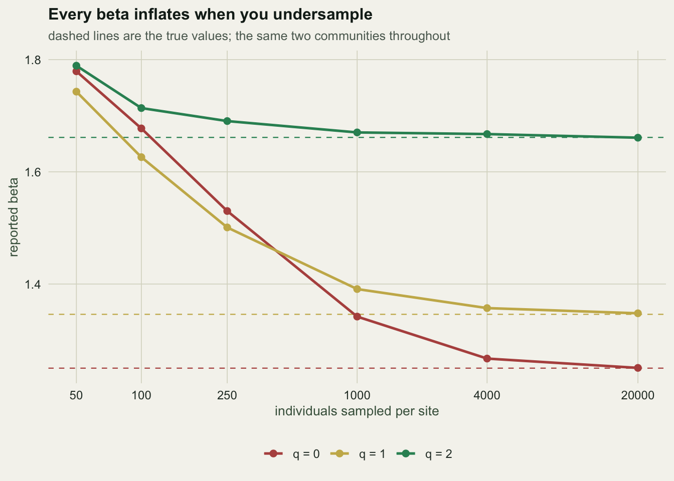
The true values are 1.250, 1.346 and 1.661. The last three columns give the bias: how far the reported beta sits above the truth, in per cent.
At 50 individuals per site, coverage is 0.49 and the reported betas are 42%, 29% and 8% too high at q = 0, 1 and 2. Every order inflates, and the inflation is lightest at q = 2. The mechanism is the one you would guess: undersampling produces unseen rare species, q = 0 counts every unseen species as a genuine absence, and a genuine absence is turnover. At q = 2 the answer is carried by the dominant species, and you have those after fifty individuals.
The ordering of the three biases belongs to this pair, not to beta diversity in general. In variants of the same construction that are not shown here, with every species equally abundant or with the site-unique species rare, the q = 2 bias can exceed the q = 0 bias, so check the ordering on a design like your own before you rely on it.
One warning about how to normalise this. It is tempting to express the bias as a multiple of the true turnover excess, (reported - 1) / (true - 1), because that reads as “you reported three times the turnover that exists”. Do not: when the true beta is close to 1 the denominator is tiny and the ratio explodes. The plain relative bias above is the honest statistic.
Equal effort is not enough
The obvious fix is to sample both regions equally hard. It does not work, and the reason is worth ten minutes.
Build two regions with identical true beta by construction: 60 species shared between the two sites, 40 unique to each. That fixes gamma at 140 and mean alpha at 100, so beta_0 is exactly 1.4 in both, whatever the abundances are, because beta_0 does not look at abundances. Then give one region an even abundance distribution and the other a heavy-tailed one:
mk_region <- function(shape) {
  co <- rlnorm(60, 0, shape); u1 <- rlnorm(40, 0, shape); u2 <- rlnorm(40, 0, shape)
  p1 <- c(co, u1, rep(0, 40)); p2 <- c(co, rep(0, 40), u2)
  rbind(p1 / sum(p1), p2 / sum(p2))
}
set.seed(1414)
PX <- mk_region(0.3)     # region X: even
PY <- mk_region(2.6)     # region Y: heavy-tailed

draw_beta0 <- function(P, m) {
  y <- rbind(rmultinom(1, m, P[1, ])[, 1], rmultinom(1, m, P[2, ])[, 1])
  keep <- colSums(y) > 0
  c(beta0 = beta_mult(y[, keep, drop = FALSE], 0),
    coverage = mean(c(good_turing(y[1, ]), good_turing(y[2, ]))),
    seen = mean(rowSums(y > 0)),
    shared_seen = sum(colSums(y[, 1:60, drop = FALSE] > 0) == 2) / 60)   # of the 60 truly shared
}

set.seed(1515)
cmp <- rbind(
  data.frame(region = "X (even)",         t(rowMeans(replicate(300, draw_beta0(PX, 200))))),
  data.frame(region = "Y (heavy-tailed)", t(rowMeans(replicate(300, draw_beta0(PY, 200))))))
cmp$true_beta0 <- c(beta_mult(PX * 1e7, 0), beta_mult(PY * 1e7, 0))
knitr::kable(cmp, digits = c(0, 3, 3, 1, 2, 4), row.names = FALSE,
             col.names = c("region", "reported beta (q = 0)", "coverage", "species seen (per site, of 100)",
"shared species detected", "true beta (q = 0)"))| region | reported beta (q = 0) | coverage | species seen (per site, of 100) | shared species detected | true beta (q = 0) |
|---|---|---|---|---|---|
| X (even) | 1.494 | 0.867 | 83.8 | 0.71 | 1.4 |
| Y (heavy-tailed) | 1.650 | 0.942 | 27.4 | 0.16 | 1.4 |
Same number of sites, same number of individuals, same true beta of 1.4 in both. Region Y reports 10% more turnover than region X. The true difference is zero.
Now look at the coverage column, because it does not say what you expect. Region Y, the one with the more inflated beta, has the higher coverage: 0.94 against X’s 0.87. It also detected 27 species against X’s 84, and it found 16% of the 60 truly shared species against X’s 71%.
That is the whole mechanism in one row. Coverage is the proportion of individuals that belong to a detected species. Region Y’s handful of dominants buy that cheaply: catch the top few species and 94% of your individuals are accounted for, while 73 of the 100 species at a site are still invisible. And beta_0 is driven by the shared species you failed to detect, which is a fact about species, not individuals.
So high coverage did not protect region Y. It was a symptom of the very tail that was hiding its shared species.
set.seed(99)
probe <- t(replicate(30, {
  P <- mk_region(runif(1, 0.2, 2.8))                 # 30 regions, tails from even to very heavy
  o <- rowMeans(replicate(60, draw_beta0(P, 200)))
  c(coverage = unname(o["coverage"]), shared_detected = unname(o["shared_seen"]),
    bias = unname(100 * (o["beta0"] / 1.4 - 1)))
}))

c(cor_coverage_with_bias        = cor(probe[, "coverage"], probe[, "bias"]),
  cor_shared_detected_with_bias = cor(probe[, "shared_detected"], probe[, "bias"]))
cor_coverage_with_bias cor_shared_detected_with_bias
0.5716653 -0.7958467 Across thirty regions that all have a true beta_0 of exactly 1.4, the correlation between coverage and beta bias is +0.57. Positive. Higher coverage goes with a more inflated beta, because in this family of communities coverage rises with tail weight and tail weight is what hides the shared species. The fraction of shared species actually detected correlates at -0.80, and that is the quantity doing the work.
Read this carefully, because it is easy to over-generalise. Within one community, coverage behaves exactly as advertised: the effort table above shows coverage climbing from 0.49 to 1.00 while bias falls to zero. Coverage is a fine measure of how complete your sample of this community is. What it will not do is make two communities with different abundance structures comparable on beta_0, and that is exactly the comparison most beta diversity papers are making.
If you find yourself writing “region Y showed higher turnover”, this is the alternative explanation, and neither equal effort nor equal coverage ruled it out.
Does coverage standardisation fix it?
The standard answer to unequal coverage is Chao and Jost (2012): compare at equal coverage rather than equal size. Try it, and be honest about what happens.
cov_at <- function(x, k) {                         # expected coverage of a subsample of size k
  n <- sum(x); if (k >= n) return(good_turing(x))
  x <- x[x > 0]
  1 - sum((x / n) * exp(lchoose(n - x, k) - lchoose(n - 1, k)))
}
k_for <- function(x, target) {
  n <- sum(x); if (good_turing(x) < target) return(NA_integer_)
  ks <- seq(5, n, by = 5); ks[which.min(abs(sapply(ks, cov_at, x = x) - target))]
}
subsample <- function(x, k) tabulate(sample(rep(seq_along(x), x), k), nbins = length(x))

std_draw <- function(P, target) {
  y  <- rbind(rmultinom(1, 8000, P[1, ])[, 1], rmultinom(1, 8000, P[2, ])[, 1])
  ys <- rbind(subsample(y[1, ], k_for(y[1, ], target)), subsample(y[2, ], k_for(y[2, ], target)))
  keep <- colSums(ys) > 0
  c(beta0 = beta_mult(ys[, keep, drop = FALSE], 0), n_used = mean(rowSums(ys)),
    seen = mean(rowSums(ys > 0)))
}

set.seed(17)
std <- do.call(rbind, lapply(c(0.80, 0.90, 0.95, 0.99), function(tg) {
  X <- rowMeans(replicate(80, std_draw(PX, tg))); Y <- rowMeans(replicate(80, std_draw(PY, tg)))
  data.frame(target_coverage = tg, X_beta0 = X["beta0"], X_individuals = X["n_used"], X_seen = X["seen"],
             Y_beta0 = Y["beta0"], Y_individuals = Y["n_used"], Y_seen = Y["seen"],
             gap_pct = 100 * (Y["beta0"] / X["beta0"] - 1))
}))
knitr::kable(std, digits = c(2, 3, 0, 1, 3, 0, 1, 0), row.names = FALSE,
             col.names = c("target coverage", "X beta", "X individuals", "X species seen",
"Y beta", "Y individuals", "Y species seen", "gap"))| target coverage | X beta | X individuals | X species seen | Y beta | Y individuals | Y species seen | gap |
|---|---|---|---|---|---|---|---|
| 0.80 | 1.534 | 155 | 76.3 | 1.743 | 30 | 11.3 | 14 |
| 0.90 | 1.472 | 230 | 87.2 | 1.729 | 92 | 19.4 | 17 |
| 0.95 | 1.441 | 312 | 93.3 | 1.651 | 238 | 29.8 | 15 |
| 0.99 | 1.411 | 519 | 98.5 | 1.515 | 1340 | 52.5 | 7 |
At a target coverage of 0.80 the two regions differ by 14%, against 10% at equal size. At the highest target tried, 0.99, the gap is 7%. The true difference is still zero at every row of that table.
The two “species seen” columns say why, and it is the same mechanism as before. At a target coverage of 0.80, region Y needs only 30 individuals against X’s 155, because a handful of dominants carry 80% of its mass. At that point Y has seen 11 species against X’s 76.
None of this is an argument against Chao and Jost (2012), which was built to make richness comparisons well defined and does that. It is an argument against expecting a standardisation designed for one quantity to fix a different quantity. For beta_0, matching coverage is not enough on its own, which means: sample harder, or report q = 0 and q = 2 side by side with the coverage behind them and say which you trust.
Check two: the metric
Two regions, eight sites each. Region A is musical chairs: the same 24 species everywhere, but a different one dominates at each site. Region B has 20 species everywhere at equal abundance, plus 4 species unique to each site.
set.seed(3072)
region_A <- t(sapply(1:8, function(i) { y <- rep(6, 24); y[i * 3] <- 300; y }))   # same list, different king
region_B <- t(sapply(1:8, function(i) {                                            # different lists, flat
  y <- numeric(20 + 8 * 4); y[1:20] <- 40; y[20 + ((i - 1) * 4 + 1):((i - 1) * 4 + 4)] <- 40; y
}))

bd_total <- function(Y) { Z <- sqrt(Y / rowSums(Y)); C <- sweep(Z, 2, colMeans(Z)); sum(C^2) / (nrow(Y) - 1) }
sorensen_mean <- function(Y) {
  X <- Y > 0
  mean(combn(nrow(Y), 2, function(p) {
    a <- sum(X[p[1], ] & X[p[2], ]); 2 * a / (sum(X[p[1], ]) + sum(X[p[2], ]))
  }))
}

verdict <- data.frame(
  metric = c("beta (q = 0)", "beta (q = 1)", "beta (q = 2)", "mean Sorensen similarity", "BD total (Hellinger)"),
  region_A = c(beta_mult(region_A, 0), beta_mult(region_A, 1), beta_mult(region_A, 2),
               sorensen_mean(region_A), bd_total(region_A)),
  region_B = c(beta_mult(region_B, 0), beta_mult(region_B, 1), beta_mult(region_B, 2),
               sorensen_mean(region_B), bd_total(region_B)))
verdict$more_beta_diverse <- ifelse(
  verdict$metric == "mean Sorensen similarity",
  ifelse(verdict$region_A < verdict$region_B, "A", "B"),
  ifelse(verdict$region_A > verdict$region_B, "A", "B"))
knitr::kable(verdict, digits = 4, row.names = FALSE,
col.names = c("metric", "region A", "region B", "which is more beta diverse?"))| metric | region A | region B | which is more beta diverse? |
|---|---|---|---|
| beta (q = 0) | 1.0000 | 2.1667 | B |
| beta (q = 1) | 3.1463 | 1.4142 | A |
| beta (q = 2) | 5.9769 | 1.1707 | A |
| mean Sorensen similarity | 1.0000 | 0.8333 | B |
| BD total (Hellinger) | 0.5049 | 0.1667 | A |
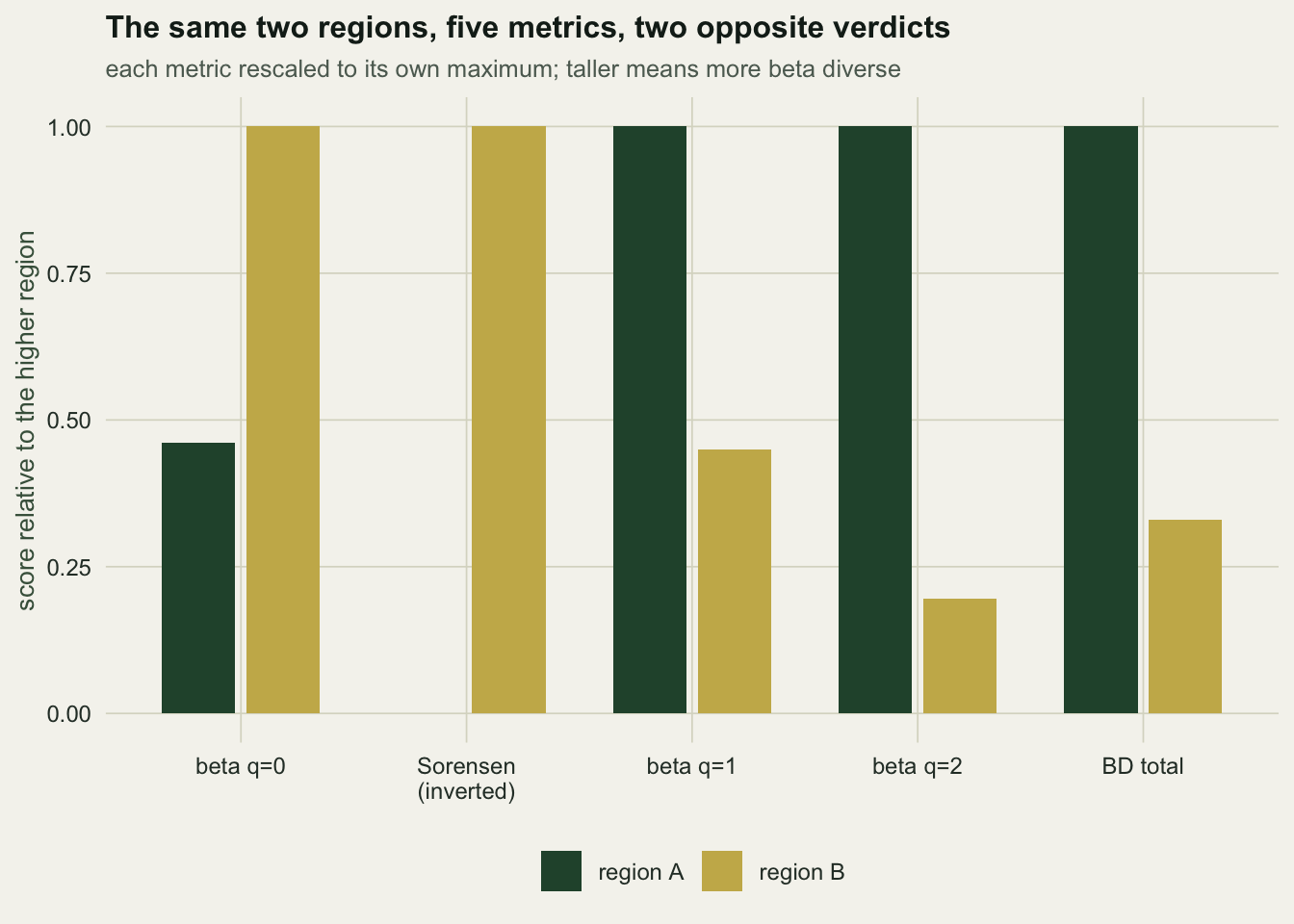
Region A’s beta_0 is exactly 1.0000 and its mean Sorensen is exactly 1.0000: on incidence data, region A has no beta diversity whatsoever. Its beta_2 is 5.98 out of a ceiling of 8. Region B is the mirror image.
There is no tie-break here and no metric is wrong. Incidence metrics report that A’s sites hold the same species. Abundance metrics report that A’s sites are running completely different communities with the same cast. Both statements are true. “Region A has more beta diversity” is not a statement about the data until you say which one you meant.
Check three: the site set
LCBD, BD and zeta are all defined relative to the set of sites you chose. Change the set and every number moves, including the ones you already published.
lcbd <- function(Y) { Z <- sqrt(Y / rowSums(Y)); C <- sweep(Z, 2, colMeans(Z)); rowSums(C^2) / sum(C^2) }

set.seed(2020)
S2 <- 50
opt <- seq(-0.15, 1.15, length.out = S2)
mk_site <- function(g) rpois(S2, 60 * exp(-((g - opt)^2) / (2 * 0.18^2)))
Y1 <- t(sapply(seq(0, 1, length.out = 12), mk_site))
rownames(Y1) <- paste0("G", 1:12)
L1 <- lcbd(Y1)

drop_one <- do.call(rbind, lapply(c(1, 6, 12), function(d) {
  Y2 <- Y1[-d, ]; L2 <- lcbd(Y2)
  data.frame(dropped = rownames(Y1)[d],
             BD_before = bd_total(Y1), BD_after = bd_total(Y2),
             top_before = names(which.max(L1[-d])), top_after = names(which.max(L2)),
             rank_spearman = cor(rank(-L1[-d]), rank(-L2), method = "spearman"))
}))
knitr::kable(drop_one, digits = c(0, 4, 4, 0, 0, 3), row.names = FALSE,
             col.names = c("site removed", "BD before", "BD after", "most unique before",
"most unique after", "rank correlation"))| site removed | BD before | BD after | most unique before | most unique after | rank correlation |
|---|---|---|---|---|---|
| G1 | 0.4416 | 0.4103 | G12 | G2 | 0.918 |
| G6 | 0.4416 | 0.4648 | G12 | G1 | 0.982 |
| G12 | 0.4416 | 0.4080 | G1 | G11 | 0.918 |
Removing one site out of twelve changes which site is the most distinctive in all three cases tried here: each end and the middle. The overall ranking barely moves (rank correlations of at least 0.918), so this is not instability in general. It is specific: LCBD finds the edges of your sampled space, and removing an edge promotes its neighbour. Removing the middle site (G6) even pushes BD up, from 0.4416 to 0.4648, because the remaining sites are more spread out without it.
Now add six more sites, which is what happens when a study expands. They draw on the same 50 species with a second set of optima, so they are not a compositionally separate habitat: on incidence, the new sites resemble the original twelve about as closely as the original twelve resemble each other.
set.seed(2121)
opt2 <- seq(1.6, 2.8, length.out = S2)
Y3 <- rbind(Y1, t(sapply(seq(1.8, 2.6, length.out = 6),
                         function(g) rpois(S2, 60 * exp(-((g - opt2)^2) / (2 * 0.18^2))))))
rownames(Y3) <- c(rownames(Y1), paste0("H", 1:6))
L3 <- lcbd(Y3)

c(BD_12_sites = bd_total(Y1), BD_18_sites = bd_total(Y3),
  LCBD_sum_of_original_12 = sum(L3[1:12]),
  G1_LCBD_before = L1["G1"], G1_LCBD_after = L3["G1"],
  rank_correlation_among_the_original_12 = cor(rank(-L1), rank(-L3[1:12]), method = "spearman"))
BD_12_sites BD_18_sites
0.4416162 0.4073982
LCBD_sum_of_original_12 G1_LCBD_before.G1
0.7023141 0.1425068
G1_LCBD_after.G1 rank_correlation_among_the_original_12
0.1010490 0.9930070 The original twelve sites now hold 0.70 of the total LCBD instead of 1, and every one of their values fell. Site G1 dropped from 0.1425 to 0.1010. Their relative ranking survived (0.993), which is the good news, but the absolute numbers are not comparable to the published ones, and BD fell from 0.4416 to 0.4074 even though the study now holds half again as many sites. BD is a variance per degree of freedom, so more sites do not lower it by themselves: the six new sites added 6 to the denominator but on average only 0.345 per site to the sum of squares, less than the original BD.
The same applies to the multiplicative beta, whose ceiling is the site count:
c(beta0_12_sites = beta_mult(Y1, 0), ceiling_12 = 12,
  beta0_18_sites = beta_mult(Y3, 0), ceiling_18 = 18,
  overlap_12 = (12 - beta_mult(Y1, 0)) / 11,       # the N-normalised version
  overlap_18 = (18 - beta_mult(Y3, 0)) / 17)
beta0_12_sites ceiling_12 beta0_18_sites ceiling_18 overlap_12
1.4563107 12.0000000 1.4084507 18.0000000 0.9585172
overlap_18
0.9759735 The raw beta went down when the study grew by six sites. The overlap transformation, which divides out the ceiling, went up. Only one of those two is comparable across the change, and it is not the one people report.
What to report
- Coverage and observed richness, next to every beta. Coverage alone is not enough, as the measurement above shows: report the species count beside it, and if you have any handle on the size of the species pool, report what fraction of it you saw.
- The order q, or the coefficient, as a decision with a reason. Not a default. If you have abundances, report at least q = 0 and q = 2; if they disagree, that disagreement is a result. In the effort table q = 2 is the order undersampling has the least grip on, but that ordering depends on the abundance structure of the pair, and nothing here tests it across two regions that differ in evenness, so do not lean on q = 2 to rescue that comparison.
- N, beside any multiplicative beta or LCBD. Multiplicative beta is bounded by it, and LCBD values average one over it.
- The species pool your sites were drawn from. LCBD and BD are relative to it.
Honest limits
These checks find artefacts, not truth. Passing all three does not make a beta correct. It rules out the three ways it is most often wrong.
No null model fixes a metric that answers the wrong question. A permutation test on beta_0 tells you whether your incidence pattern is unlikely by chance. It cannot tell you that you should have looked at abundances, and it will happily hand you a small p value while you do the wrong thing. The variance framing post has a worked case where the permutation test certifies an artefact at p = 0.002.
Everything here assumes the sites are the sampling unit. If sites are nested inside regions, or repeated in time, the whole design question comes back and none of these one-table checks address it.
Undersampling usually inflates beta, but the sign is not free. Thin effort separates sites when the species they share are the ones most easily missed, which is the case the effort table shows. Turn that around, with the shared species abundant and the site-unique ones rare, and at moderate effort a richness-based beta moves the other way: the unique species are the ones still missing, so the sites look more alike than they are. Thin that same design far enough and the shared species start dropping out too, and it inflates again. Thinning the site set rather than the sampling within sites can push BD either way as well, as check three shows. Work out which shape your data has before you lean on the sign of a bias.
References
Chao & Jost 2012 Ecology 93(12):2533-2547 (10.1890/11-1952.1)
Chao, Gotelli, Hsieh, Sander, Ma, Colwell & Ellison 2014 Ecological Monographs 84(1):45-67 (10.1890/13-0133.1)
Jost 2007 Ecology 88(10):2427-2439 (10.1890/06-1736.1)
Legendre & De Caceres 2013 Ecology Letters 16(8):951-963 (10.1111/ele.12141)