library(ggplot2)

theme_te <- function() {
  theme_minimal(base_size = 12) +
    theme(plot.background  = element_rect(fill = "#f5f4ee", colour = NA),
          panel.background = element_rect(fill = "#f5f4ee", colour = NA),
          panel.grid.minor = element_blank(),
          panel.grid.major = element_line(colour = "#dad9ca", linewidth = 0.3),
          plot.title    = element_text(colour = "#16241d", face = "bold", size = 12),
          plot.subtitle = element_text(colour = "#5d6b61", size = 9.5),
          axis.title    = element_text(colour = "#46604a", size = 10),
          axis.text     = element_text(colour = "#2c3a31", size = 9),
          legend.text   = element_text(colour = "#2c3a31", size = 9),
          legend.title  = element_text(colour = "#46604a", size = 9.5))
}Multiplicative beta diversity with Hill numbers
R
beta diversity
biodiversity
Hill numbers
ecology tutorial
Why additive Gini-Simpson beta is capped by one minus alpha, how Jost’s alpha fixes it, and the exact identity that turns Hill beta into the Sorensen index.
Corrected 14 October 2026: the description said additive Gini-Simpson beta is bounded by alpha; it now says it is capped by one minus alpha, as the text argues.
Corrected 1 October 2026: the post said the additive beta of two communities is scored out of a possible one, that a small additive beta shows only that alpha was large, and that the naive alpha is always too big by a gap set by evenness; it now gives the ceiling of one half, says a small additive beta cannot tell low turnover from a large alpha, and says the naive alpha is too big whenever the per-site diversities differ, by more as they spread apart through richness or evenness.
Here are two communities. The first holds 100 species, evenly abundant. The second holds 100 different species, evenly abundant. They share nothing at all: not one species.
Now measure their beta diversity. The additive Gini-Simpson partition says 0.005. Jost’s multiplicative partition says 2.000. Tilt the pair so the second community holds one species instead of 100, and a multiplicative partition built on the arithmetic mean of the two Simpson diversities returns 0.078: a beta below one for two communities that still share nothing.
All three are computed correctly. Only Jost’s is a number you can interpret, and the reason is worth an afternoon.
Setup
Nothing beyond base R and ggplot2. The house theme keeps the figures consistent with the rest of the blog.
The three quantities
A Hill number of order q is the effective number of species: how many equally abundant species would give the diversity you observe. The order q sets how much a rare species counts. This blog has covered the alpha side of that (Hill numbers and the diversity profile, estimating them); here they do beta duty.
hill <- function(p, q) {
  p <- p[p > 0]
  if (abs(q - 1) < 1e-10) return(exp(-sum(p * log(p))))
  sum(p^q)^(1 / (1 - q))
}

sum_pq <- function(p, q) { p <- p[p > 0]; sum(p^q) }   # the zero mask matters: 0^0 is 1 in R

gamma_hill <- function(Y, q) hill(colMeans(Y / rowSums(Y)), q)   # pooled, equal weights
Gamma is easy: pool the sites with equal weights and take the Hill number. Alpha is where the trouble lives, and beta is defined by whatever alpha you chose, because beta is gamma divided by alpha.
Trap one: additive beta on the Gini-Simpson index
The additive partition writes gamma as alpha plus beta, where alpha is the mean of the per-site index and gamma is the index of the pooled data. It is the classical move, and this blog has a post on it (additive diversity partitioning). Applied to the Gini-Simpson index (one minus the sum of squared proportions), it does something strange.
Take N = 2 communities with S even species each and nothing shared. Vary S.
gini <- function(p) 1 - sum(p^2)

mk_distinct <- function(S, N = 2) {          # N communities, S species each, zero overlap
  Y <- matrix(0, N, N * S)
  for (i in 1:N) Y[i, ((i - 1) * S + 1):(i * S)] <- 1
  Y
}

add_gs <- function(Y) {
  P <- Y / rowSums(Y)
  gini(colMeans(P)) - mean(apply(P, 1, gini))
}

S_grid <- c(5, 10, 25, 50, 100)
tab1 <- data.frame(
  S        = S_grid,
  shared   = 0L,
  beta_add = sapply(S_grid, function(S) add_gs(mk_distinct(S))),
  formula  = 1 / (2 * S_grid)
)
tab1$abs_gap <- abs(tab1$beta_add - tab1$formula)

# a gap this small is floating-point rounding, so the tables say it in words
gap_text <- function(g) {
  stopifnot(all(g < 1e-10))
  ifelse(g == 0, "0", "rounding only")
}
knitr::kable(transform(tab1, abs_gap = gap_text(abs_gap)), digits = c(0, 0, 6, 6, 20),
             col.names = c("S per site", "shared species", "additive Gini-Simpson beta",
"1/(2S)", "gap"))| S per site | shared species | additive Gini-Simpson beta | 1/(2S) | gap |
|---|---|---|---|---|
| 5 | 0 | 0.100 | 0.100 | rounding only |
| 10 | 0 | 0.050 | 0.050 | rounding only |
| 25 | 0 | 0.020 | 0.020 | rounding only |
| 50 | 0 | 0.010 | 0.010 | rounding only |
| 100 | 0 | 0.005 | 0.005 | rounding only |
The measured additive beta is 1/(2S) to within floating-point rounding (the gap column), and the algebra is a two-liner: alpha is 1 - 1/S, gamma is 1 - 1/(2S), and the difference is 1/(2S).
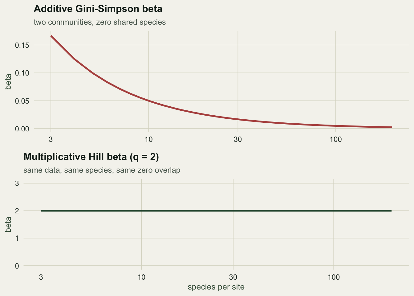
So with 100 species per site and zero overlap, the additive Gini-Simpson beta is 0.005. Two communities with nothing in common score 0.005, on an index that can never exceed one half for two equally weighted communities. The number is not wrong, it is bounded: the Gini-Simpson index cannot exceed 1, so once alpha is close to 1 there is no room left for beta. A small additive beta therefore cannot tell low turnover from a large alpha.
Now the multiplicative version of the same data:
alpha_jost <- function(Y, q) {
  P <- Y / rowSums(Y)
  if (abs(q - 1) < 1e-10)
    return(exp(mean(apply(P, 1, function(p) { p <- p[p > 0]; -sum(p * log(p)) }))))
  mean(apply(P, 1, sum_pq, q = q))^(1 / (1 - q))
}

beta_mult <- function(Y, q) gamma_hill(Y, q) / alpha_jost(Y, q)

tab1$beta_hill_q2 <- sapply(S_grid, function(S) beta_mult(mk_distinct(S), 2))
knitr::kable(tab1[, c("S", "beta_add", "beta_hill_q2")], digits = c(0, 6, 10),
col.names = c("S per site", "additive Gini-Simpson beta", "multiplicative Hill beta (q = 2)"))| S per site | additive Gini-Simpson beta | multiplicative Hill beta (q = 2) |
|---|---|---|
| 5 | 0.100 | 2 |
| 10 | 0.050 | 2 |
| 25 | 0.020 | 2 |
| 50 | 0.010 | 2 |
| 100 | 0.005 | 2 |
Flat at 2, for every richness. Two completely distinct communities are two communities. That is the whole claim of the multiplicative partition, and it is why Jost (2007) called the result the effective number of distinct communities: the number is on the same scale as the thing being counted.
Trap two: the alpha that looks obvious
If beta is gamma over alpha, and alpha is the average within-site diversity, then surely alpha is the mean of the per-site Hill numbers. Try it on a lopsided pair: one site with 100 even species, one site with a single species, nothing shared.
Y2 <- matrix(0, 2, 101)
Y2[1, 1:100] <- 1     # site A: 100 even species
Y2[2, 101]   <- 1     # site B: one species, and it is not in A

per_site  <- apply(Y2 / rowSums(Y2), 1, hill, q = 2)
g2        <- gamma_hill(Y2, 2)
a_naive   <- mean(per_site)          # arithmetic mean of the per-site Hill numbers
a_correct <- alpha_jost(Y2, 2)

c(site_A = per_site[1], site_B = per_site[2],
  gamma = g2, alpha_naive = a_naive, alpha_jost = a_correct,
  beta_naive = g2 / a_naive, beta_jost = g2 / a_correct)
site_A site_B gamma alpha_naive alpha_jost beta_naive
100.00000000 1.00000000 3.96039604 50.50000000 1.98019802 0.07842368
beta_jost
2.00000000 The naive route reports a beta diversity of 0.0784 for two communities that share not one species. A beta below 1 is not a large or a small answer, it is an impossible one: gamma came out lower than the average within-site diversity.
The correct alpha is 1.9802, and it is not the arithmetic mean of 100 and 1. It is the harmonic mean:
c(alpha_jost = a_correct, harmonic_mean = 1 / mean(1 / per_site),
  gap = abs(a_correct - 1 / mean(1 / per_site)))
alpha_jost harmonic_mean gap
1.980198 1.980198 0.000000 The rule behind it
Jost’s alpha, with equal site weights, is the power mean of order 1 - q of the per-site Hill numbers. At q = 0 that is order 1, the plain arithmetic mean of richness, which is why nobody ever noticed a problem there. At q = 2 it is order -1, the harmonic mean. At q = 1 it is the limit, the exponential of the mean Shannon entropy.
set.seed(304)
Yr <- matrix(rpois(6 * 40, 3), 6, 40)          # six sites, forty species

pm_check <- do.call(rbind, lapply(c(0, 0.5, 2, 3), function(q) {
  ds <- apply(Yr / rowSums(Yr), 1, hill, q = q)
  data.frame(q = q, order = 1 - q,
             alpha_jost  = alpha_jost(Yr, q),
             power_mean  = mean(ds^(1 - q))^(1 / (1 - q)))
}))
pm_check$gap <- abs(pm_check$alpha_jost - pm_check$power_mean)
knitr::kable(transform(pm_check, gap = gap_text(gap)), digits = c(1, 1, 8, 8, 20),
col.names = c("q", "mean order (1 - q)", "Jost alpha", "power mean of per-site Hill numbers", "gap"))| q | mean order (1 - q) | Jost alpha | power mean of per-site Hill numbers | gap |
|---|---|---|---|---|
| 0.0 | 1.0 | 38.00000 | 38.00000 | 0 |
| 0.5 | 0.5 | 35.34457 | 35.34457 | 0 |
| 2.0 | -1.0 | 29.61492 | 29.61492 | 0 |
| 3.0 | -2.0 | 26.96940 | 26.96940 | rounding only |
Identical at all four orders, down to floating-point rounding in the last bits.
This also explains why the arithmetic mean fails at q = 2: the power mean of order -1 is never larger than the arithmetic mean, so the naive alpha is too big, and the naive beta too small, whenever the per-site diversities differ. The gap widens as they spread apart, whether through richness or evenness, which is when you most wanted the answer.
What beta is allowed to be
With equal weights, beta runs from 1 to N and hits both ends exactly.
range_tab <- do.call(rbind, lapply(c(2, 3, 5, 8), function(N) {
  Y_dist <- mk_distinct(20, N)                # N communities, nothing shared
  Y_same <- matrix(1, N, 20)                  # N identical communities
  data.frame(N = N,
             distinct_q0 = beta_mult(Y_dist, 0), distinct_q1 = beta_mult(Y_dist, 1),
             distinct_q2 = beta_mult(Y_dist, 2),
             identical_q1 = beta_mult(Y_same, 1), identical_q2 = beta_mult(Y_same, 2))
}))
knitr::kable(range_tab, digits = 10,
             col.names = c("N", "distinct, q=0", "distinct, q=1", "distinct, q=2",
"identical, q=1", "identical, q=2"))| N | distinct, q=0 | distinct, q=1 | distinct, q=2 | identical, q=1 | identical, q=2 |
|---|---|---|---|---|---|
| 2 | 2 | 2 | 2 | 1 | 1 |
| 3 | 3 | 3 | 3 | 1 | 1 |
| 5 | 5 | 5 | 5 | 1 | 1 |
| 8 | 8 | 8 | 8 | 1 | 1 |
N completely distinct communities give beta exactly N. N identical communities give exactly 1. Every order of q agrees, because the replication property is what the effective-number scale was built to satisfy.
That upper bound of N is also the catch: beta is not comparable between a study with 5 sites and a study with 40 unless you convert it first. More on that in a moment.
The bridge to the additive world
Shannon is the one index where the additive and multiplicative accounts are the same statement in different clothing:
P  <- Yr / rowSums(Yr)
Hs <- apply(P, 1, function(p) { p <- p[p > 0]; -sum(p * log(p)) })
Hg <- { p <- colMeans(P); p <- p[p > 0]; -sum(p * log(p)) }

c(log_beta_mult = log(beta_mult(Yr, 1)),
  H_gamma_minus_H_alpha = Hg - mean(Hs),
  gap = abs(log(beta_mult(Yr, 1)) - (Hg - mean(Hs))))
log_beta_mult H_gamma_minus_H_alpha gap
0.1526125 0.1526125 0.0000000 The additive Shannon beta is the logarithm of the multiplicative beta, exactly. This is the reason the additive partition kept its reputation: on Shannon entropy it works, and everyone generalised from the one case where nothing goes wrong. Jost (2007) shows the harder half of the same result: when site weights are unequal, Shannon is the only standard measure that still decomposes into an alpha and a beta that behave.
Turning beta into an overlap
Because beta tops out at N, comparing raw betas across studies compares the number of sites. The fix is a transformation to an overlap measure on [0, 1], and the payoff is that these are not new inventions: they are the indices ecologists were already using.
CqN <- function(beta, q, N) {
  if (abs(q - 1) < 1e-10) return(1 - log(beta) / log(N))
  ((1 / beta)^(q - 1) - (1 / N)^(q - 1)) / (1 - (1 / N)^(q - 1))
}

set.seed(3041)
sor_check <- do.call(rbind, lapply(1:5, function(i) {
  a <- sample(2:20, 1); b <- sample(1:20, 1); cc <- sample(1:20, 1)
  Y <- matrix(0, 2, a + b + cc)
  Y[1, 1:(a + b)] <- 1                                # a shared, b only in A
  Y[2, c(1:a, (a + b + 1):(a + b + cc))] <- 1         # a shared, c only in B
  data.frame(a = a, b = b, c = cc,
             beta_q0  = beta_mult(Y, 0),
             C_02     = CqN(beta_mult(Y, 0), 0, 2),
             sorensen = 2 * a / (2 * a + b + cc))
}))
sor_check$gap <- abs(sor_check$C_02 - sor_check$sorensen)
knitr::kable(transform(sor_check, gap = gap_text(gap)), digits = c(0, 0, 0, 6, 10, 10, 20))| a | b | c | beta_q0 | C_02 | sorensen | gap |
|---|---|---|---|---|---|---|
| 6 | 10 | 14 | 1.666667 | 0.3333333 | 0.3333333 | rounding only |
| 5 | 6 | 8 | 1.583333 | 0.4166667 | 0.4166667 | rounding only |
| 16 | 8 | 7 | 1.319149 | 0.6808511 | 0.6808511 | rounding only |
| 2 | 20 | 5 | 1.862069 | 0.1379310 | 0.1379310 | rounding only |
| 18 | 13 | 1 | 1.280000 | 0.7200000 | 0.7200000 | 0 |
The Sorensen index is the q = 0 overlap transformation of the multiplicative beta for two sites. Not approximately: in all five random cases the two agree to within floating-point rounding. Push q to 2 and the same transformation gives you Morisita-Horn:
set.seed(3042)
mh_check <- do.call(rbind, lapply(1:4, function(i) {
  Y <- matrix(rpois(2 * 12, 4), 2, 12)
  Y[1, sample(12, 3)] <- 0; Y[2, sample(12, 3)] <- 0
  Pm <- Y / rowSums(Y)
  data.frame(beta_q2 = beta_mult(Y, 2),
             C_22 = CqN(beta_mult(Y, 2), 2, 2),
             morisita_horn = 2 * sum(Pm[1, ] * Pm[2, ]) / (sum(Pm[1, ]^2) + sum(Pm[2, ]^2)))
}))
mh_check$gap <- abs(mh_check$C_22 - mh_check$morisita_horn)
knitr::kable(transform(mh_check, gap = gap_text(gap)), digits = c(6, 10, 10, 20))| beta_q2 | C_22 | morisita_horn | gap |
|---|---|---|---|
| 1.179949 | 0.6949887 | 0.6949887 | rounding only |
| 1.324720 | 0.5097528 | 0.5097528 | rounding only |
| 1.232448 | 0.6227866 | 0.6227866 | rounding only |
| 1.270646 | 0.5740026 | 0.5740026 | 0 |
So the classical similarity indices were never a separate tradition. They are the multiplicative beta, rescaled by N, read at different q. Jaccard and Horn fall out of the same family.
q is a decision, and it moves the answer
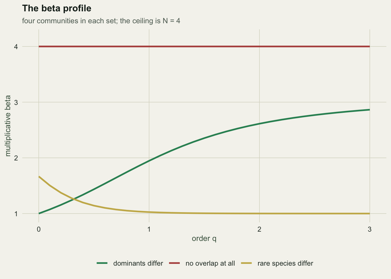
| site set | beta (q = 0) | beta (q = 1) | beta (q = 2) |
|---|---|---|---|
| rare species differ | 1.667 | 1.026 | 1.001 |
| dominants differ | 1.000 | 1.947 | 2.613 |
At q = 0 the set whose rare species differ scores 1.67 against 1.00, so it wins. At q = 2 it scores 1.00 against 2.61, and it loses. Nothing about the data changed. The order q is a question about what you think turnover is, and the profile is the honest way to report it: one curve, not one number.
Honest limits
Equal weights. Everything above assumes the sites carry equal weight. Jost (2007) shows that with unequal weights the general q decomposition breaks: alpha can come out larger than gamma, which is nonsense, and only the Shannon case (q = 1) survives intact. If your sites differ in area or effort, either weight them equally on purpose and say so, or stay at q = 1.
The ceiling is N. Raw beta lives in [1, N]. A beta of 3 means something different in a 4-site study and a 40-site study. Report the overlap transformation, or report N beside beta and never compare the raw values across designs.
The effective number is not a count of anything real. A beta of 2.4 does not mean there are between two and three communities out there. It means the assemblage is as differentiated as 2.4 equally weighted, completely distinct communities would be. That is a yardstick, not a census.
Sampling. Every number here came from complete knowledge of the communities. Real beta comes from samples, and samples bias it. That is a separate post: checking a beta diversity analysis.
Where to go next
The multiplicative partition answers “how many communities’ worth of difference is there”. It is not the only sensible question. If you want to ask how many species several sites share at once, the pairwise and multiplicative framings both fall short, and zeta diversity picks up the thread. If you want to ask which site is contributing the difference, the variance framing gives you a per-site number: beta diversity as variance.
And if you take one thing: check what your beta is bounded by before you interpret its size. A low beta diversity result is worth checking against its own alpha before it is believed.
References
Jost 2007 Ecology 88(10):2427-2439 (10.1890/06-1736.1)
Jost 2006 Oikos 113(2):363-375 (10.1111/j.2006.0030-1299.14714.x)
Tuomisto 2010 Ecography 33:2-22 (10.1111/j.1600-0587.2009.05880.x)
Chao, Gotelli, Hsieh, Sander, Ma, Colwell & Ellison 2014 Ecological Monographs 84(1):45-67 (10.1890/13-0133.1)