library(ggplot2)

te_pal <- list(forest = "#275139", green = "#2f8f63", sage = "#93a87f",
               clay = "#b5534e", gold = "#cda23f", line = "#dad9ca",
               ink = "#16241d", paper = "#f5f4ee")

theme_te <- function() {
  theme_minimal(base_size = 12) +
    theme(panel.grid.minor = element_blank(),
          panel.grid.major = element_line(colour = "#e7e6dc"),
          plot.background = element_rect(fill = "#f5f4ee", colour = NA),
          panel.background = element_rect(fill = "#f5f4ee", colour = NA),
          plot.title = element_text(face = "bold", colour = te_pal$ink),
          axis.title = element_text(colour = "#2c3a31"),
          legend.position = "bottom")
}Checking a macroecological pattern
R
macroecology
model checking
ecology tutorial
ggplot2
Four checks on a macroecological pattern in R: the shared record set, a random placement null, non-independent species, and slopes that move with grain.
The recording scheme has forty years of records on one grid. Somebody exports the lot, counts how many cells each species was recorded in, divides each species’ record total by its number of occupied cells, and plots one against the other on log axes. The cloud slopes upwards. Widespread species are locally commoner, restricted species are locally scarcer, and the line through the middle has an R squared that would pass any reviewer. A mechanism gets attached to it within a paragraph: niche breadth, or metapopulation dynamics, or a density dependent habitat selection argument.
The plot has a property that the mechanism talk skips over. Both axes came out of the same table. Occupancy is the number of cells with at least one record. Mean abundance is the record total divided by the number of cells with at least one record. Nothing in the figure was measured independently of anything else in the figure, and the atlas that produced it was assembled by volunteers whose effort was not designed around either quantity.
This post runs four checks on that plot and puts a number on each. The first asks how much of the relationship a record set with no relationship in it will produce anyway. The second builds the null model that has to run before any slope means anything, and tests it on a case where it must pass as well as a case where it must fail. The third asks how many independent data points 240 species really are. The fourth recomputes the same slope across a grid of grains and extents and reports how far it moves.
The data are simulated throughout, for the usual reason: a simulated atlas comes with a truth column, so a spurious correlation can be measured against a known zero rather than argued about. Two companion posts fit the patterns that this one attacks. The abundance-occupancy relationship fits the pattern and works through what it can and cannot mean, and range size distributions does the same job for the distribution of range sizes across species. Two further posts own ideas that this one uses without re-deriving: closure and spurious correlation sets out how ratios built from a shared total generate correlation in compositional data, and phylogenetic generalised least squares handles non-independence across species properly, by modelling the covariance rather than resampling it. Read either of those first if the idea is new; what follows is about the macroecological estimator, not about the general result.
Check 1: both axes come out of the same records
The cleanest way to measure a spurious correlation is to build a world where the true correlation is zero and see what the estimator returns. Here 150 species live on 100 atlas cells. Each species gets a true occupancy drawn uniformly between 0.05 and 0.85, and a true local density drawn log uniformly between 0.15 and 3 records per cell visit, and the two draws are independent. Every cell is visited six times. In a cell the species genuinely occupies, each visit turns up a Poisson number of records with the species’ own mean; in a cell it does not occupy, no visit turns up anything. No false positives, no effort gradient, no spatial structure. This is the friendliest atlas that has ever existed.
From that record set the two conventional quantities are formed: occupancy is the share of cells with at least one record, and mean abundance is the record total divided by the number of occupied cells. Both are logged, as they always are, and the correlation across species is taken. Whatever that correlation is, it is not ecology, because there is no ecology in the generator to find.
Seven variants of the calculation are run on the same records. Two use the conventional recipe on different amounts of effort. One divides the record total by every cell rather than by the occupied ones, which is the correction people usually reach for first. One takes the occupancy from the first two visits and the abundance from the next two, so that no record appears on both axes. One deliberately breaks the numerator and denominator apart: it divides the visits 3 and 4 record total by the visits 1 and 2 cell count, which is the textbook ratio artefact with nothing to cancel it. The last two use an occupancy that has been corrected for detection, and the true occupancy, which nobody has.
set.seed(20260725)
n_cell <- 100L
n_spp <- 150L
n_vis <- 6L
n_rep <- 200L
c(species = n_spp, cells = n_cell, visits_per_cell = n_vis, replicates = n_rep)
species cells visits_per_cell replicates
150 100 6 200 p_grid <- seq(1e-4, 1 - 1e-6, length.out = 4000)
m_grid <- n_vis * p_grid / (1 - (1 - p_grid)^n_vis)
atlas <- function() {
psi <- runif(n_spp, 0.05, 0.85)
lam <- exp(runif(n_spp, log(0.15), log(3)))
z <- matrix(rbinom(n_spp * n_cell, 1, psi), n_spp, n_cell)
zl <- z * lam
tot <- hits <- aa <- bb <- matrix(0, n_spp, n_cell)
for (v in seq_len(n_vis)) {
yv <- matrix(rpois(n_spp * n_cell, zl), n_spp, n_cell)
tot <- tot + yv
hits <- hits + (yv > 0)
if (v <= 2L) aa <- aa + yv else if (v <= 4L) bb <- bb + yv
}
oc <- rowSums(tot > 0)
md <- rowSums(hits) / pmax(oc, 1)
ph <- approx(m_grid, p_grid, xout = pmin(pmax(md, m_grid[1]), max(m_grid)),
rule = 2)$y
list(psi = psi, lam = lam, o_all = oc, n_all = rowSums(tot),
o_a = rowSums(aa > 0), n_a = rowSums(aa),
o_b = rowSums(bb > 0), n_b = rowSums(bb),
o_true = rowSums(z),
psi_hat = pmin((oc / n_cell) / (1 - (1 - ph)^n_vis), 1),
keep = oc >= 2 & rowSums(aa > 0) >= 2 & rowSums(bb > 0) >= 2)
}
cors <- function(d) {
k <- d$keep
c(truth = cor(log(d$lam[k]), log(d$psi[k])),
six_visits = cor(log(d$n_all[k] / d$o_all[k]), log(d$o_all[k] / n_cell)),
two_visits = cor(log(d$n_a[k] / d$o_a[k]), log(d$o_a[k] / n_cell)),
all_cells = cor(log(d$n_all[k] / n_cell), log(d$o_all[k] / n_cell)),
split_halves = cor(log(d$n_b[k] / d$o_b[k]), log(d$o_a[k] / n_cell)),
shared_denom = cor(log(d$n_b[k] / d$o_a[k]), log(d$o_a[k] / n_cell)),
detection_corrected = cor(log(d$n_all[k] / d$o_all[k]), log(d$psi_hat[k])),
true_occupancy = cor(log(d$n_all[k] / d$o_all[k]), log(d$o_true[k] / n_cell)))
}
rr <- t(replicate(n_rep, cors(atlas())))
ao_tab <- cbind(mean = colMeans(rr), t(apply(rr, 2, quantile, c(0.025, 0.975))))
print(round(ao_tab, 4)) mean 2.5% 97.5%
truth -0.0332 -0.1951 0.1266
six_visits 0.1270 -0.0345 0.2846
two_visits 0.4213 0.2672 0.5472
all_cells 0.7283 0.6409 0.7888
split_halves 0.4222 0.2718 0.5415
shared_denom 0.3354 0.2105 0.4585
detection_corrected -0.0533 -0.2098 0.1125
true_occupancy -0.0321 -0.2023 0.1321round(c(shared_denominator_effect = ao_tab["two_visits", "mean"] -
ao_tab["split_halves", "mean"],
pure_ratio_effect = ao_tab["shared_denom", "mean"] -
ao_tab["split_halves", "mean"],
detection_effect = ao_tab["split_halves", "mean"] -
ao_tab["true_occupancy", "mean"]), 4)shared_denominator_effect pure_ratio_effect detection_effect
-0.0009 -0.0868 0.4543 demo <- atlas()
kd <- demo$keep
q_lam <- quantile(demo$lam, c(0.25, 0.75))
round(c(occ_ratio_low_density = mean((demo$o_all / (n_cell * demo$psi))[
kd & demo$lam < q_lam[1]]),
occ_ratio_high_density = mean((demo$o_all / (n_cell * demo$psi))[
kd & demo$lam > q_lam[2]]),
species_used = sum(kd)), 4) occ_ratio_low_density occ_ratio_high_density species_used
0.7384 0.9596 149.0000 Start with the row that has no estimation in it. The correlation between true log density and true log occupancy averages -0.0332 over 200 replicate atlases, with a central 95 per cent range from -0.1951 to 0.1266. That is the zero this check is measured against.
The conventional recipe on all six visits returns 0.1270. On two visits it returns 0.4213, with the lower end of its 95 per cent range at 0.2672, so ninety-five per cent of the 200 replicate atlases returned a clearly positive correlation on a generator that contains none. The size of the artefact is set by survey effort rather than by anything living in the cells, and a pattern that gets weaker the more often each cell is visited is a property of the recording.
Now the shared denominator, which is the usual suspect. Occupancy is the cell count, and mean abundance is a record total divided by that same cell count, so the two should be tied together by the noise they share. Holding the occupancy axis fixed at the visits 1 and 2 cell count and swapping the abundance from those same two visits to the independent visits 3 and 4 changes the correlation by -0.0009. That is nothing. The suspect has an alibi, and the alibi is the numerator: the record total is built out of the same records as the cell count, so when a species happens to be found in more cells than usual it also happens to have more records than usual, and the two errors cancel in the ratio.
The artefact appears the moment that cancellation is removed. Dividing the visits 3 and 4 record total by the visits 1 and 2 cell count leaves a denominator shared with the x axis and a numerator that knows nothing about it, and the correlation drops to 0.3354 from 0.4222, a shift of -0.0868. So the ratio artefact is real, it is measurable, and in this setting it is negative: it works against the pattern rather than for it. That is the opposite of what I set out to demonstrate, and it is worth stating plainly, because the compositional case in closure and spurious correlation does bite hard, and the difference is whether the numerator carries the denominator’s noise.
The correction people reach for first is worse than the problem. Dividing the record total by every cell instead of by the occupied ones gives 0.7283. It has to: mean abundance over all cells is local density multiplied by occupancy, so occupancy is now sitting on both axes by construction rather than by accident. Wilson (2011) works through the consequences of that choice of mean, and the number here is the reason a plot of this kind should always say which mean it used.
pan <- function(x, y, lab) data.frame(x = x, y = y, panel = lab)
sc_df <- rbind(
  pan(log10(demo$psi[kd]), log10(demo$lam[kd] * n_vis),
      "1. The truth: independent by construction"),
  pan(log10(demo$o_all[kd] / n_cell), log10(demo$n_all[kd] / demo$o_all[kd]),
      "2. Records: mean over occupied cells"),
  pan(log10(demo$o_all[kd] / n_cell), log10(demo$n_all[kd] / n_cell),
      "3. Records: mean over all cells"),
  pan(log10(demo$psi_hat[kd]), log10(demo$n_all[kd] / demo$o_all[kd]),
      "4. Detection corrected occupancy"))
sc_df$panel <- factor(sc_df$panel, levels = unique(sc_df$panel))

ggplot(sc_df, aes(x, y)) +
  geom_point(colour = te_pal$green, alpha = 0.65, size = 1.5) +
  geom_smooth(method = "lm", formula = y ~ x, se = FALSE,
              colour = te_pal$clay, linewidth = 0.9) +
  facet_wrap(~panel) +
  labs(x = "log10 occupancy", y = "log10 mean abundance",
       title = "The same atlas, four ways of reading it") +
  theme_te() +
  theme(strip.text = element_text(colour = te_pal$ink, face = "bold", size = 9),
        plot.margin = margin(6, 12, 6, 6))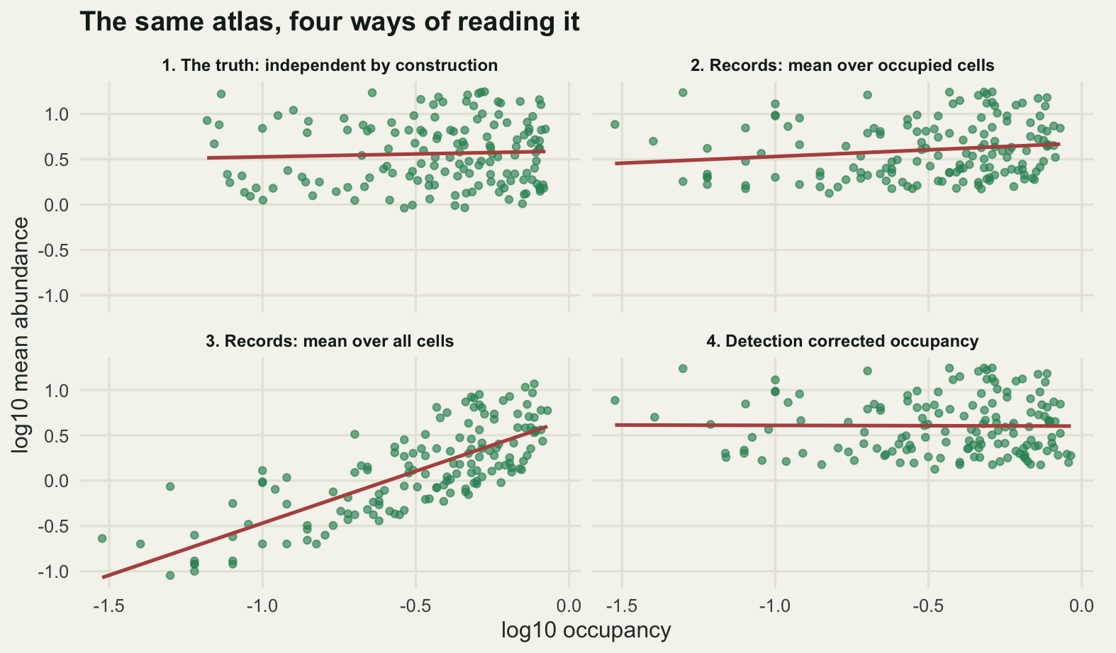
The bottom right panel says where the artefact actually lives. Occupancy estimated from records is biased downwards, because a species can be present in a cell and go unrecorded, and the size of that bias depends on local density. In the atlas drawn here, the quarter of species with the lowest density recover 0.7384 of their true occupancy, while the quarter with the highest density recover 0.9596 of it. The x axis is compressed at the scarce end by an amount that is a function of the y axis. That is the whole pattern.
Correcting for it is not hard here. Each cell was visited six times, so for every species the number of visits that produced a record in an occupied cell follows a zero truncated binomial, and matching its mean gives a per visit detection probability; dividing the raw occupancy by the probability of being found at least once undoes the compression. That estimator returns -0.0533, against -0.0321 when the true occupancy is handed over. The detection channel is worth 0.4543 of correlation on this design and the ratio channel is worth -0.0868; the detection one is the part that survey effort shrinks, which is what the gap between the two_visits and six_visits rows of the table above shows. Verdict: the shared denominator is not what breaks a macroecological scatter plot, and the axis to defend is occupancy, not the ratio.
Check 2: the null model that has to run first
A slope of zero is not the interesting hypothesis. If every individual of every species were thrown at the grid at random, the abundant species would still occupy more cells than the scarce ones, and a plot of mean abundance against occupancy would still slope upwards, because both are functions of the same total. The question a macroecological pattern has to answer is not whether the slope differs from zero but whether it differs from what random placement would give with the same totals on the same grid. Wright (1991) put that argument in print for incidence and abundance.
That null is easy to build. Keep each species’ record total exactly as observed, scatter those records over the cells with equal probability, recompute occupancy and mean abundance, refit the slope. Repeat. The distribution of null slopes is the yardstick.
A check that cannot fail is not a check, so the null is run on two datasets. In the first the individuals really were placed at random, so the null has to pass. In the second they were placed with negative binomial clumping, so the null has to reject. Both use 120 species on a 256 cell grid with the same distribution of totals.
set.seed(20260726)
n_c2 <- 256L
n_s2 <- 120L
n_null <- 400L
clump_k <- 0.4
c(species = n_s2, cells = n_c2, null_replicates = n_null)
species cells null_replicates
120 256 400 print(c(clumping_parameter = clump_k))clumping_parameter
0.4 ao_slope <- function(nn, oo, n) {
k <- oo >= 2 & oo < n
unname(coef(lm(log(nn[k] / oo[k]) ~ log(oo[k] / n)))[2])
}
occ_random <- function(m) sum(as.vector(rmultinom(1, m, rep(1, n_c2))) > 0)
null_slope <- function(m) ao_slope(m, vapply(m, occ_random, numeric(1)), n_c2)
tot_r <- round(exp(runif(n_s2, log(10), log(1200))))
occ_r <- vapply(tot_r, occ_random, numeric(1))
agg <- t(sapply(tot_r, function(m) rnbinom(n_c2, mu = m / n_c2, size = clump_k)))
tot_a <- rowSums(agg)
occ_a <- rowSums(agg > 0)
s_r <- ao_slope(tot_r, occ_r, n_c2)
s_a <- ao_slope(tot_a, occ_a, n_c2)
null_r <- replicate(n_null, null_slope(tot_r))
null_a <- replicate(n_null, null_slope(tot_a))
nul_tab <- rbind(
"random placement data" = c(observed = s_r, null_mean = mean(null_r),
quantile(null_r, c(0.025, 0.975)),
n_null_ge_obs = sum(null_r >= s_r)),
"aggregated data" = c(observed = s_a, null_mean = mean(null_a),
quantile(null_a, c(0.025, 0.975)),
n_null_ge_obs = sum(null_a >= s_a)))
print(round(nul_tab, 4)) observed null_mean 2.5% 97.5% n_null_ge_obs
random placement data 0.3276 0.3342 0.3229 0.3433 348
aggregated data 0.5995 0.3391 0.3275 0.3485 0round(c(observed_over_null_random = s_r / mean(null_r),
observed_over_null_aggregated = s_a / mean(null_a),
occupancy_max_random = max(occ_r) / n_c2,
occupancy_max_aggregated = max(occ_a) / n_c2,
smallest_total = min(tot_r), largest_total = max(tot_r)), 4) observed_over_null_random observed_over_null_aggregated
0.9803 1.7679
occupancy_max_random occupancy_max_aggregated
1.0000 0.6797
smallest_total largest_total
10.0000 1194.0000 k_r <- occ_r >= 2 & occ_r < n_c2
naive <- summary(lm(log(tot_r[k_r] / occ_r[k_r]) ~ log(occ_r[k_r] / n_c2)))
round(c(naive_slope = unname(naive$coefficients[2, 1]),
naive_t_against_zero = unname(naive$coefficients[2, 3]),
naive_r_squared = naive$r.squared,
species_used = sum(k_r)), 4) naive_slope naive_t_against_zero naive_r_squared
0.3276 14.8670 0.6539
species_used
119.0000 Take the negative control first. On records that were placed at random, the fitted slope is 0.3276 and the null distribution runs from 0.3229 to 0.3433 with a mean of 0.3342. The observation sits inside its own null, which is what had to happen, and the fact that it did is the only reason to believe anything the null says about the second dataset.
The same data destroy the conventional test. Fitting the ordinary regression and testing the slope against zero gives a t statistic of 14.87 on 119 species with an R squared of 0.6539. That is as convincing as a macroecological result ever looks, on data generated by throwing individuals at a grid. The relationship is entirely real and entirely uninteresting: it is the arithmetic of putting 10 to 1194 items into 256 boxes.
On the aggregated data the slope is 0.5995, against a null mean of 0.3391 and an upper null limit of 0.3485. None of the 400 null replicates reached the observed value, so the null is rejected at the resolution the replication allows, and the observed slope is 1.7679 times the null mean. What the rejection buys is narrow but real: the species are more aggregated than random placement, and the excess slope is a measure of how much. It does not identify why they are aggregated.
null_df <- rbind(
  data.frame(slope = null_r, case = "Records placed at random"),
  data.frame(slope = null_a, case = "Records clumped"))
obs_df <- data.frame(slope = c(s_r, s_a), hj = c(-0.12, 1.12),
                     case = c("Records placed at random", "Records clumped"))
null_df$case <- factor(null_df$case,
                       levels = c("Records placed at random", "Records clumped"))
obs_df$case <- factor(obs_df$case, levels = levels(null_df$case))

ggplot(null_df, aes(slope)) +
  geom_histogram(bins = 30, fill = te_pal$sage, colour = te_pal$forest,
                 linewidth = 0.2) +
  geom_vline(data = obs_df, aes(xintercept = slope), colour = te_pal$clay,
             linetype = "42", linewidth = 0.9) +
  geom_text(data = obs_df, aes(x = slope, y = Inf, label = "observed", hjust = hj),
            vjust = 1.6, size = 3.3, colour = te_pal$clay) +
  facet_wrap(~case, scales = "free") +
  labs(x = "Fitted abundance-occupancy slope", y = "Null replicates",
       title = "The null the slope has to beat is not zero") +
  theme_te() +
  theme(strip.text = element_text(colour = te_pal$ink, face = "bold"),
        plot.margin = margin(6, 16, 6, 6))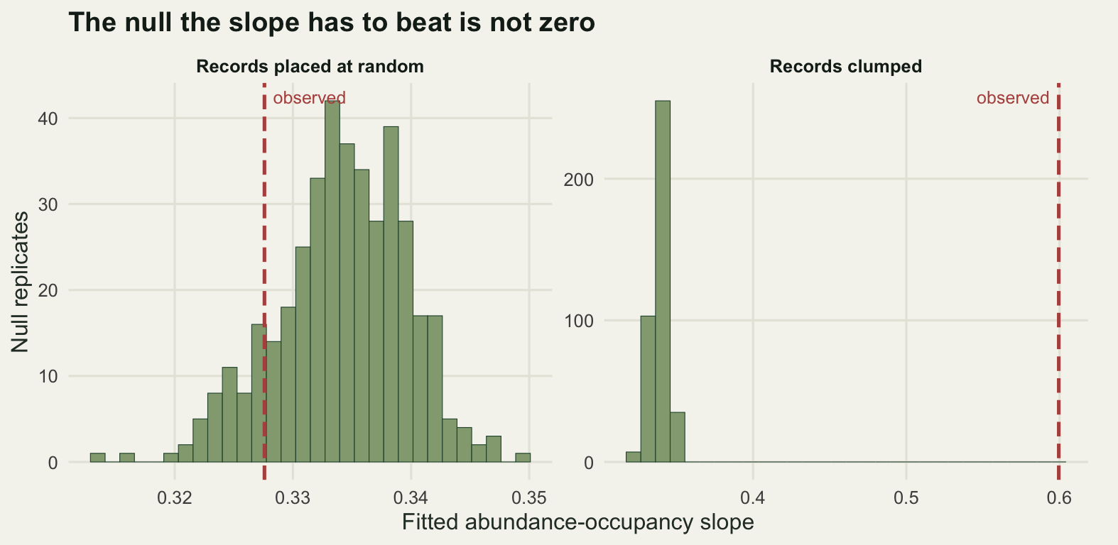
The two nulls sit in almost the same place on the slope axis, because the null depends on the record totals and the totals are similar; the panels are drawn on free scales, so the figure will not show you that. The distance between the dashed line and the mound is the entire result. Gotelli and Graves set this out for co-occurrence, and the same machinery, with the same argument about what to hold fixed, is worked through for interaction data in null models for co-occurrence. Verdict: the null costs 400 refits and it converts a slope of 0.5995, which on its own is evidence of nothing, into an excess of 0.2604 over random placement, which is a measurement.
Check 3: species are not independent data points
The scatter has one point per species and the regression treats those points as independent draws. They are not. Species in the same genus share a body size, a dispersal syndrome and a habitat, and species in the same landscape share the landscape. Both push the residuals of a macroecological regression into blocks, and a blocked residual makes the reported standard error a work of fiction while leaving the point estimate roughly alone.
The measurement is a simulation with the answer known. There are 240 species in 24 families of ten. A share rho of the variance in the predictor and a share rho of the variance in the residual are family level rather than species level, so rho is a dial running from complete independence to strong shared structure. The slope is fitted by ordinary least squares in every replicate, and the thing to compare is the standard deviation of the slope estimates actually realised against the standard error the model reports. Alongside it, a bootstrap that resamples whole families rather than species.
set.seed(20260727)
n_fam <- 24L
per_fam <- 10L
n_sp3 <- n_fam * per_fam
b_true <- 0.6
n_rep3 <- 400L
n_boot <- 199L
c(families = n_fam, species_per_family = per_fam, species = n_sp3,
  replicates = n_rep3, bootstrap_resamples = n_boot)
families species_per_family species replicates
24 10 240 400
bootstrap_resamples
199 print(c(true_slope = b_true))true_slope
0.6 fam <- rep(seq_len(n_fam), each = per_fam)
suff <- function(x, y) cbind(1, x, y, x * x, x * y, y * y)
slope_of <- function(s) (s[, 5] - s[, 2] * s[, 3] / s[, 1]) /
(s[, 4] - s[, 2] * s[, 2] / s[, 1])
one_fit <- function(rho) {
u <- rnorm(n_fam)
v <- rnorm(n_fam)
x <- sqrt(rho) * u[fam] + sqrt(1 - rho) * rnorm(n_sp3)
y <- b_true * x + sqrt(rho) * v[fam] + sqrt(1 - rho) * rnorm(n_sp3)
s <- suff(x, y)
tt <- colSums(s)
sxx <- tt[4] - tt[2]^2 / n_sp3
sxy <- tt[5] - tt[2] * tt[3] / n_sp3
syy <- tt[6] - tt[3]^2 / n_sp3
b <- sxy / sxx
se <- sqrt(((syy - b * sxy) / (n_sp3 - 2)) / sxx)
tc <- qt(0.975, n_sp3 - 2)
fs <- rowsum(s, fam)
idx <- as.vector(matrix(sample.int(n_fam, n_fam * n_boot, TRUE), n_fam, n_boot))
bs <- slope_of(rowsum(fs[idx, , drop = FALSE], rep(seq_len(n_boot), each = n_fam)))
ci <- unname(quantile(bs, c(0.025, 0.975)))
c(b = unname(b), se = unname(se),
cov_ols = unname(abs(b - b_true) <= tc * se),
cov_boot = as.numeric(b_true >= ci[1] && b_true <= ci[2]),
width_ols = unname(2 * tc * se), width_boot = ci[2] - ci[1])
}
rhos <- c(0, 0.15, 0.3, 0.5, 0.7)
fam_tab <- t(vapply(rhos, function(rho) {
m <- t(replicate(n_rep3, one_fit(rho)))
sd_b <- sd(m[, "b"])
se_b <- mean(m[, "se"])
c(rho = rho, sd_of_slope = sd_b, reported_se = se_b, ratio = sd_b / se_b,
effective_species = n_sp3 / (sd_b / se_b)^2,
coverage_ols = mean(m[, "cov_ols"]), coverage_boot = mean(m[, "cov_boot"]),
width_ols = mean(m[, "width_ols"]), width_boot = mean(m[, "width_boot"]))
}, numeric(9)))
print(round(fam_tab, 4)) rho sd_of_slope reported_se ratio effective_species coverage_ols
[1,] 0.00 0.0649 0.0650 0.9984 240.7768 0.9550
[2,] 0.15 0.0691 0.0652 1.0597 213.7238 0.9500
[3,] 0.30 0.0910 0.0648 1.4051 121.5602 0.8275
[4,] 0.50 0.1159 0.0644 1.7981 74.2283 0.7300
[5,] 0.70 0.1375 0.0643 2.1400 52.4062 0.6000
coverage_boot width_ols width_boot
[1,] 0.9150 0.2563 0.2395
[2,] 0.9425 0.2568 0.2611
[3,] 0.9050 0.2553 0.3154
[4,] 0.9125 0.2539 0.4123
[5,] 0.9250 0.2532 0.5458With rho at zero the machinery is calibrated, which is the check on the check: the realised standard deviation of the slope is 0.0649 against a reported standard error of 0.0650, a ratio of 0.9984, and the nominal 95 per cent interval covers the true slope in 0.9550 of replicates.
Turn the dial to a rho of 0.50 and the reported standard error is 0.0644 while the slope actually varies with a standard deviation of 0.1159, a ratio of 1.7981. Coverage falls to 0.7300. Since precision scales with the square root of the sample size, that ratio implies an effective sample of 74.2 species where the table says 240. At a rho of 0.70 the effective sample is 52.4 species, and 40.0 intervals in every hundred miss the true slope where five were supposed to.
pan_cov <- "Coverage of the 95 per cent interval: both methods"
pan_rat <- "Realised spread over reported error: least squares only"
cov_df <- rbind(
  data.frame(rho = fam_tab[, "rho"], value = fam_tab[, "coverage_ols"],
             method = "Ordinary least squares", panel = pan_cov),
  data.frame(rho = fam_tab[, "rho"], value = fam_tab[, "coverage_boot"],
             method = "Block bootstrap over families", panel = pan_cov),
  data.frame(rho = fam_tab[, "rho"], value = fam_tab[, "ratio"],
             method = "Ordinary least squares", panel = pan_rat))
cov_df$panel <- factor(cov_df$panel, levels = c(pan_cov, pan_rat))
ref_df <- data.frame(panel = factor(c(pan_cov, pan_rat),
                                    levels = c(pan_cov, pan_rat)),
                     y = c(0.95, 1))

ggplot(cov_df, aes(rho, value, colour = method, shape = method)) +
  geom_hline(data = ref_df, aes(yintercept = y), colour = te_pal$ink,
             linetype = "22", linewidth = 0.5) +
  geom_line(linewidth = 0.9) +
  geom_point(size = 2.1) +
  facet_wrap(~panel, scales = "free_y") +
  scale_colour_manual(values = c(te_pal$gold, te_pal$forest), name = NULL) +
  scale_shape_manual(values = c(17, 16), name = NULL) +
  labs(x = "Share of variance shared within families", y = NULL,
       title = "Shared history empties the confidence interval") +
  theme_te() +
  theme(strip.text = element_text(colour = te_pal$ink, face = "bold", size = 9),
        plot.margin = margin(6, 14, 6, 6))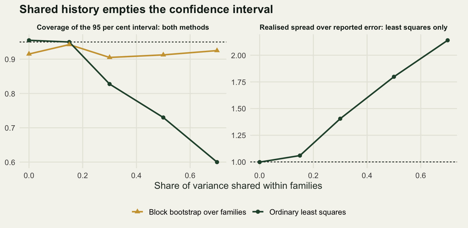
The bootstrap that resamples families rather than species does most of the repair. Its coverage runs from 0.9050 to 0.9425 across the whole sweep, against 0.6000 for the least squares interval at the strongest structure, and it gets there by widening: at a rho of 0.70 its mean width is 0.5458 against 0.2532. It is not exact. Even at a rho of zero it covers 0.9150, because a percentile interval built from 24 blocks is a little too narrow, and that residual error is the price of resampling something with 24 units in it. The right tool when the shared structure is a phylogeny is to model the covariance directly, which is phylogenetic generalised least squares; the general problem of resampling data that come in blocks is bootstrapping dependent data, and the reason the count of rows is not the count of independent observations is pseudoreplication in ecology. Freckleton (2009) lists this among the recurring failures of comparative analysis, and it is the one that changes conclusions rather than decimal places. Verdict: the slope needs no repair and the interval needs all of it, so quote the block bootstrap interval and read the sample size as 52.4 species rather than 240 whenever the shared structure is strong.
Check 4: grain and extent, run as a sweep
The last check is the one most often handled with a sentence in the methods. A macroecological slope is computed on cells of some size within a region of some size, and both choices were made by whoever drew the recording grid. If the slope moves when they move, then a slope quoted without them is not a quantity.
The landscape here is 128 units on a side and holds 90 species placed as clusters: each species gets a number of cluster centres, a spread around them, and a total number of individuals, all drawn independently of each other. The pattern is recomputed on cells of 1, 2, 4 and 8 units within nested subregions of 128, 64 and 32 units, giving twelve fitted slopes from one landscape. A second landscape uses the same abundance distribution but gives every species the same number of centres and the same spread, so that only total abundance differs between species.
set.seed(20260728)
side <- 128L
n_sp4 <- 90L
grains <- c(1L, 2L, 4L, 8L)
exts <- c(128L, 64L, 32L)
c(species = n_sp4, landscape_side = side)
species landscape_side
90 128 print(c(grains = grains))grains1 grains2 grains3 grains4
1 2 4 8 print(c(extents = exts))extents1 extents2 extents3
128 64 32 make_land <- function(vary) {
tot <- round(exp(runif(n_sp4, log(150), log(9000))))
if (vary) {
npar <- round(exp(runif(n_sp4, log(4), log(60))))
sprd <- exp(runif(n_sp4, log(1.2), log(6)))
} else {
npar <- rep(15L, n_sp4)
sprd <- rep(3, n_sp4)
}
xx <- numeric(0); yy <- numeric(0); id <- integer(0)
for (i in seq_len(n_sp4)) {
px <- runif(npar[i], 0, side)
py <- runif(npar[i], 0, side)
j <- sample.int(npar[i], tot[i], TRUE)
xx <- c(xx, (px[j] + rnorm(tot[i], 0, sprd[i])) %% side)
yy <- c(yy, (py[j] + rnorm(tot[i], 0, sprd[i])) %% side)
id <- c(id, rep(i, tot[i]))
}
list(x = xx, y = yy, id = id, total = tot)
}
cells_of <- function(w, grain, ext) {
k <- w$x < ext & w$y < ext
m <- as.integer(ext / grain)
cid <- as.integer(w$x[k] %/% grain) + as.integer(w$y[k] %/% grain) * m
matrix(tabulate(w$id[k] + n_sp4 * cid, n_sp4 * m * m), n_sp4, m * m)
}
scale_fit <- function(w, grain, ext) {
cm <- cells_of(w, grain, ext)
nc <- ncol(cm)
oo <- rowSums(cm > 0)
nn <- rowSums(cm)
k <- oo >= 2 & oo < nc
c(slope = unname(coef(lm(log(nn[k] / oo[k]) ~ log(oo[k] / nc)))[2]),
species = sum(k), cells = nc)
}
grid_of <- function(w, what) {
z <- outer(grains, exts, Vectorize(function(g, e) scale_fit(w, g, e)[what]))
dimnames(z) <- list(paste("grain", grains), paste("extent", exts))
z
}
land_v <- make_land(TRUE)
land_c <- make_land(FALSE)
c(individuals_varying = length(land_v$x), individuals_constant = length(land_c$x)) individuals_varying individuals_constant
238356 219794 slope_v <- grid_of(land_v, "slope")
slope_c <- grid_of(land_c, "slope")
print(round(slope_v, 4)) extent 128 extent 64 extent 32
grain 1 0.2581 0.2219 0.2149
grain 2 0.1557 0.2076 0.2578
grain 4 -0.1148 -0.0356 0.2045
grain 8 -0.2708 -0.1872 0.3792print(grid_of(land_v, "species")) extent 128 extent 64 extent 32
grain 1 90 90 72
grain 2 90 90 72
grain 4 90 89 71
grain 8 90 89 66print(round(slope_c, 4)) extent 128 extent 64 extent 32
grain 1 0.4408 0.3550 0.2529
grain 2 1.1670 0.7716 0.5189
grain 4 2.5000 1.1694 0.8778
grain 8 4.0776 1.1344 0.9755round(c(varying_min = min(slope_v), varying_max = max(slope_v),
varying_span = max(slope_v) - min(slope_v),
constant_min = min(slope_c), constant_max = max(slope_c),
constant_ratio = max(slope_c) / min(slope_c)), 4) varying_min varying_max varying_span constant_min constant_max
-0.2708 0.3792 0.6500 0.2529 4.0776
constant_ratio
16.1251 # each panel of the figure below also has to hold the zero line, so the vertical
# span a reader sees is the range of the slopes together with zero
panel_span_v <- diff(range(c(slope_v, 0)))
panel_span_c <- diff(range(c(slope_c, 0)))
panel_span_ratio <- panel_span_c / panel_span_v
round(c(panel_span_varying = panel_span_v, panel_span_constant = panel_span_c,
panel_span_ratio = panel_span_ratio), 4) panel_span_varying panel_span_constant panel_span_ratio
0.6500 4.0776 6.2732 occ_at <- function(w, grain, ext) {
cm <- cells_of(w, grain, ext)
rowSums(cm > 0) / ncol(cm)
}
round(c(rank_fine_vs_coarse_grain = cor(occ_at(land_v, 1L, 128L),
occ_at(land_v, 8L, 128L),
method = "spearman"),
rank_full_vs_quarter_extent = cor(occ_at(land_v, 2L, 128L),
occ_at(land_v, 2L, 32L),
method = "spearman")), 4) rank_fine_vs_coarse_grain rank_full_vs_quarter_extent
0.6532 0.6232 The first table is the result. Across the twelve combinations the fitted slope runs from -0.2708 to 0.3792, a span of 0.6500, and it changes sign. At the finest cells the pattern is the familiar positive one at every extent. At the coarsest cells over the whole landscape it is -0.2708: widespread species are locally scarcer, which is the opposite claim, from the same individuals, on the same day. Quoting a ratio between the largest and smallest slope here would be dishonest arithmetic, because the two have different signs; the span is the honest summary.
The second landscape says what the sign flip needs. When every species has the same clustering and only total abundance differs, the slope never changes sign: it runs from 0.2529 to 4.0776, a factor of 16.1251 across the same twelve combinations. So the magnitude is scale dependent whatever the species do, and the sign becomes scale dependent as soon as species differ in how clumped they are, which they always do. At coarse grain a tightly clustered species is squeezed into few cells with many individuals in each, and that pushes the point up and to the left; at fine grain the same species looks like everything else.
melt_grid <- function(z, lab) data.frame(
  grain = rep(grains, times = length(exts)),
  extent = factor(rep(exts, each = length(grains)),
                  levels = exts, labels = paste(exts, "units")),
  slope = as.vector(z), land = lab)
sw_df <- rbind(
  melt_grid(slope_v, "Species differ in clustering"),
  melt_grid(slope_c, "All species clustered alike"))
sw_df$land <- factor(sw_df$land, levels = c("Species differ in clustering",
                                            "All species clustered alike"))

ggplot(sw_df, aes(grain, slope, colour = extent, shape = extent)) +
  geom_hline(yintercept = 0, colour = te_pal$ink, linetype = "22",
             linewidth = 0.5) +
  geom_line(linewidth = 0.9) +
  geom_point(size = 2.2) +
  facet_wrap(~land, scales = "free_y") +
  scale_x_continuous(transform = "log2", breaks = grains) +
  scale_colour_manual(values = c(te_pal$forest, te_pal$gold, te_pal$clay),
                      name = "Extent") +
  scale_shape_manual(values = c(16, 17, 15), name = "Extent") +
  labs(x = "Cell size (units)", y = "Fitted slope",
       title = "The slope is a property of the grid as much as the species") +
  theme_te() +
  theme(strip.text = element_text(colour = te_pal$ink, face = "bold", size = 9),
        plot.margin = margin(6, 14, 6, 6))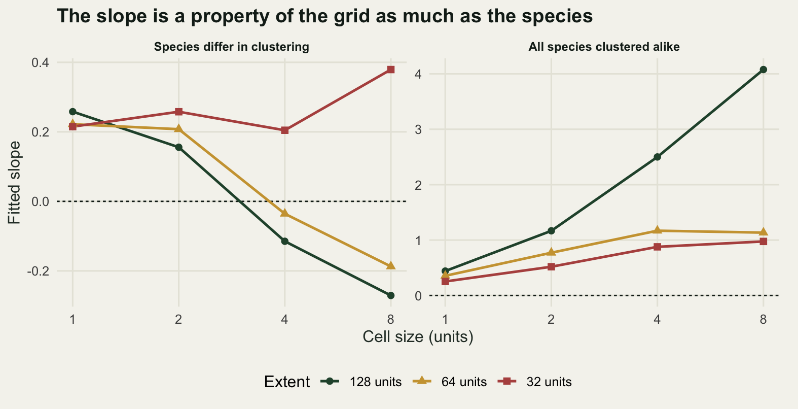
Something does survive the sweep, and it is worth naming because it is what the analysis can actually deliver. The rank order of species by occupancy at the finest cells and at the coarsest correlates at 0.6532 by Spearman, and between the full extent and the quarter extent at the same grain it is 0.6232. Neither is high enough to call the ranking stable, but both are far more stable than the coefficient, which changed sign. A statement of the form “these species are the widespread ones” survives a change of grid better than a statement of the form “the slope is 0.3”, and papers routinely report the second and rely on the first. Rahbek (2005) made the same argument for richness patterns, and species-area relationships is the case where the scale dependence is the subject rather than the nuisance. Verdict: a slope quoted without its grain and its extent is not a quantity, and on this landscape the two conventions available to an honest analyst differ by 0.6500 and by their sign.
Which check catches what
The four checks fail on different things and none substitutes for another.
Check 1 catches an artefact of the recording, and it is the one to run when the pattern is strongest in the least well recorded taxa. It would not have caught the aggregation in check 2, because the records there were complete. Check 2 catches a slope that is only the arithmetic of totals, and it is the one to run before any mechanism is proposed. It would reject the check 1 atlas too, because records lost to imperfect detection shrink occupancy for a given record total in the same direction that clumping does, and it would report that rejection as aggregation. That is the reason check 1 runs first: the null says the records are more concentrated than random placement, never why. Check 3 catches nothing about the point estimate at all and everything about the interval, so it changes whether a difference between two taxa or two decades is real; the other three checks would have passed a dataset that check 3 fails. Check 4 catches a result that exists only at the grain someone happened to choose, and it is the cheapest of the four to run on an existing analysis, because it needs no simulation, only the same code on a coarser grid.
If only one can be run, run check 4. It requires nothing that is not already on the machine, and in the landscape above it flipped the sign.
The honest limit
All four checks are about the estimator. Each one asks whether a number computed from an atlas means what the arithmetic says it means, and each returns an answer with a standard error. None of them can tell you that the pattern is caused by what you think causes it.
The measurement above makes the point without any extra machinery. In check 2 the aggregated landscape rejected the random placement null at 0.5995 against a null mean of 0.3391. The generator that produced it was a negative binomial with a clumping parameter of 0.4 and nothing else: no niche breadth, no dispersal, no metapopulation, no habitat. A rejection of random placement is a statement that individuals are aggregated, and essentially every ecological mechanism ever proposed for the abundance-occupancy relationship predicts aggregation. The null separates aggregation from no aggregation, and stops there. Check 1 has the same property in the other direction: it can tell you that occupancy was underestimated for scarce species, but it cannot tell you whether the surviving relationship is niche breadth or a shared response to habitat area, since both produce the same scatter with the same slope. That degeneracy between mechanisms is the subject of the abundance-occupancy relationship, and it is not fixable by better estimation.
Two smaller limits are worth stating. The simulated landscapes here are stationary: recording effort is uniform, and no cell is better watched than any other. Real atlases are the opposite, and an effort gradient that correlates with anything ecological will produce all four pathologies at once, which is the subject of sampling bias in presence-only models. And check 3 imposes a block structure by family, which is a caricature of a phylogeny; a real tree has structure at every depth, and the effective sample size under a real tree can be lower than the block calculation suggests.
Where to go next
The cheapest thing to do with an existing macroecological result is check 4, because it costs one loop. Recompute the slope on cells twice as wide and on half the region. If the answer moves by more than the confidence interval, the interval was never the uncertainty that mattered.
After that, the null model. Any statement that a pattern is stronger than expected needs an expectation, and for atlas data the expectation is random placement of the observed totals rather than a slope of zero; null models for co-occurrence works through what to hold fixed and why the choice does most of the work. If the pattern is spatial as well, spatial autocorrelation and Moran’s I measures the dependence that check 3 only caricatures, and the same correction applies: the number of cells is not the number of independent observations.
References
Brown JH 1984 The American Naturalist 124(2):255-279 (10.1086/284267)
Wright DH 1991 Journal of Biogeography 18(4):463 (10.2307/2845487)
Gaston KJ, Blackburn TM, Greenwood JJD, Gregory RD, Quinn RM, Lawton JH 2000 Journal of Applied Ecology 37(s1):39-59 (10.1046/j.1365-2664.2000.00485.x)
Wilson PD 2011 Global Ecology and Biogeography 20(1):193-202 (10.1111/j.1466-8238.2010.00569.x)
Freckleton RP 2009 Journal of Evolutionary Biology 22(7):1367-1375 (10.1111/j.1420-9101.2009.01757.x)
Rahbek C 2005 Ecology Letters 8(2):224-239 (10.1111/j.1461-0248.2004.00701.x)
Gotelli NJ, Graves GR 1996 Null Models in Ecology, Smithsonian Institution Press (ISBN 978-1-56098-657-7)