library(ggplot2)
library(patchwork)
library(survival)

te_paper  <- "#f5f4ee"
te_ink    <- "#16241d"
te_body   <- "#2c3a31"
te_forest <- "#275139"
te_rust   <- "#b5534e"
te_gold   <- "#c9b458"
te_line   <- "#dad9ca"

theme_datasheet <- function() {
  theme_minimal(base_size = 12) +
    theme(plot.background  = element_rect(fill = te_paper, colour = NA),
          panel.background = element_rect(fill = te_paper, colour = NA),
          panel.grid.major = element_line(colour = te_line, linewidth = 0.3),
          panel.grid.minor = element_blank(),
          text             = element_text(colour = te_body),
          plot.title       = element_text(colour = te_ink, face = "bold"),
          plot.subtitle    = element_text(colour = te_body),
          axis.text        = element_text(colour = te_body))
}Rapoport’s rule and the Stevens method
R
macroecology
biogeography
range size
simulation
ecology tutorial
Stevens’ band-mean method finds Rapoport’s rule in worlds with none, and pole clipping biases the species midpoint method too. Edge treatments tested in R.
Four hundred species of a group with good range maps, each reduced to two numbers: the southern and the northern limit of its range in degrees of latitude. The difference is the latitudinal extent. The pattern people look for in such a table is Rapoport’s rule, the name Stevens gave in 1989 to the claim that species living at higher latitudes have wider latitudinal ranges. His method was simple and it spread: cut the latitude axis into bands of five degrees, list the species whose range covers each band, average their extents, and plot the band means against latitude.
Rohde, Heap and Heap objected in 1993 that the band means are not independent data. A species with a wide range is counted in every band it covers, so one wide ranging species appears in many band means at once, and a band far from the equator is reached only by the species whose ranges are long enough to get there. They proposed the midpoint method instead: each species is counted once, in the five degree band that holds the midpoint of its range, and the mean extent of those species is plotted against the latitude of the band. The species-level midpoint regression used below takes that idea to its end, one point per species, log extent against absolute midpoint latitude; it is a later variant, and the post runs Rohde’s band form next to it. Below, the midpoint method means that species-level regression unless Rohde’s band form is named. Colwell and Hurtt showed in 1994 that hard boundaries to a domain produce gradients in richness and a spurious Rapoport effect with no biology at all, and Gaston, Blackburn and Spicer reviewed the evidence in 1998 and found it largely confined to high northern latitudes. None of what follows is a new result. It is a measurement of those arguments on simulated worlds in which the true link between range size and latitude is set by hand, so each method’s error can be put next to the width of the equatorial richness peak and the typical size of a range.
This site already covers the neighbouring problems. Checking a macroecological pattern shows that species in the same family are not independent points in a cross species regression, and resamples whole families to get an honest standard error. The trouble here is a different kind of dependence: the same species entering many band means, and ranges cut short by the edge of the domain. Checking a trait environment analysis shows that a community weighted mean correlation can come back highly significant when the true trait to environment link is zero, the problem Peres-Neto, Dray and ter Braak set out in 2017. A Stevens band mean is exactly that kind of mean, a presence weighted average of one trait per site, with latitude as the site variable; the twist is that the trait, range extent, also decides which sites a species is counted in. Range size distributions measures range size itself, with grain, effort and the choice between area of occupancy and extent of occurrence, and never relates it to latitude.
The post measures four things: how often each method finds a rule in worlds that have none, as the richness peak narrows and ranges grow; what each does with a real rule of either sign; what four ways of handling clipped ranges do to the midpoint method and to Stevens’ statistic; and how continental limits, a hemisphere-only data set and an assemblage version of Bergmann’s rule fit the same picture.
A world with known ranges
The domain is one latitude axis from the south pole to the north pole. Each species gets a true midpoint and a true extent. Midpoints are drawn from a normal distribution centred on the equator and truncated at the poles, so richness peaks at the equator; the standard deviation of that normal is the width of the peak, and a uniform draw is the case with no richness gradient. Extents are lognormal. A true rule enters as a slope on absolute latitude in the log extent, per 45 degrees, so a slope of 0.5 makes a species at a pole 2.7 times as wide ranging as the same species at the equator. Then the poles cut every range that runs past them, and the observed extent and midpoint are what is left.
n_sp      <- 400                         # species per world
band_w    <- 5                           # band width, degrees
sd_log    <- 0.7                         # spread of log extent
alpha_lev <- 0.05

# equator-peaked midpoints: a normal truncated to the domain (Inf = uniform)
draw_mid <- function(n, peak_sd, edges) {
  if (is.infinite(peak_sd)) return(runif(n, edges[1], edges[2]))
  u <- runif(n, pnorm(edges[1], 0, peak_sd), pnorm(edges[2], 0, peak_sd))
  qnorm(u, 0, peak_sd)
}

# one world: true midpoint, true extent with a slope on absolute latitude, then the edges cut
make_world <- function(peak_sd = 25, ext_med = 20, rule = 0, edges = c(-90, 90)) {
  m_true <- draw_mid(n_sp, peak_sd, edges)
  ext <- ext_med * exp(rule * abs(m_true) / 45 + rnorm(n_sp, 0, sd_log))
  lo <- pmax(m_true - ext / 2, edges[1]); hi <- pmin(m_true + ext / 2, edges[2])
  list(lo = lo, hi = hi, ext = hi - lo, mid = (lo + hi) / 2, edges = edges,
       touch = lo <= edges[1] | hi >= edges[2])
}

band_centres <- function(edges) {
  b <- seq(-90 + band_w / 2, 90 - band_w / 2, by = band_w)
  b[b - band_w / 2 >= edges[1] & b + band_w / 2 <= edges[2]]
}
Stevens’ band means need, for every band centre, the number and the summed extent of the species whose range covers it. Sorting the lower and the upper limits once gives both for all bands by cumulative sums, which matters because the edge treatments further down run this calculation many thousands of times. The check is against the plain band by species matrix and against lm for the two regressions.
# Stevens: mean extent of the species whose range covers each band centre.
# Sorted cumulative sums give every band total without a band by species matrix.
stevens_means <- function(lo, hi, ext, centres) {
  o1 <- order(lo); o2 <- order(hi)
  i1 <- findInterval(centres, lo[o1])                    # species with lo <= centre
  i2 <- findInterval(centres, hi[o2], left.open = TRUE)  # species with hi <  centre
  cs1 <- c(0, cumsum(ext[o1])); cs2 <- c(0, cumsum(ext[o2]))
  n_in <- i1 - i2; tot <- cs1[i1 + 1] - cs2[i2 + 1]
  ok <- n_in > 0
  list(lat = abs(centres[ok]), mean_ext = tot[ok] / n_in[ok], n = n_in[ok])
}

# slope and two-sided t-test p value of a simple regression, no model object
slope_test <- function(x, y) {
  xc <- x - mean(x); b <- sum(xc * (y - mean(y))) / sum(xc^2)
  rss <- sum((y - mean(y) - b * xc)^2); dfr <- length(x) - 2
  se <- sqrt(rss / dfr / sum(xc^2))
  c(b = b, p = 2 * pt(-abs(b / se), dfr))
}

# Rohde, Heap and Heap: each species counted once, in the band holding its range midpoint
rohde_means <- function(mid, ext) {
  band <- floor((mid + 90) / band_w)
  band[band == 180 / band_w] <- 180 / band_w - 1         # a midpoint exactly at 90 north
  mean_ext <- tapply(ext, band, mean)
  list(lat = abs(as.numeric(names(mean_ext)) * band_w - 90 + band_w / 2),
       mean_ext = as.vector(mean_ext))
}

both_methods <- function(w, centres = band_centres(w$edges)) {
  st <- stevens_means(w$lo, w$hi, w$ext, centres)
  rh <- rohde_means(w$mid, w$ext)
  c(st = slope_test(st$lat, st$mean_ext), mp = slope_test(abs(w$mid), log(w$ext)),
    rh = slope_test(rh$lat, rh$mean_ext))
}

set.seed(1989)
w_demo <- make_world(peak_sd = 25, ext_med = 20, rule = 0)
cen <- band_centres(w_demo$edges)
st_fast <- stevens_means(w_demo$lo, w_demo$hi, w_demo$ext, cen)
cover <- outer(cen, w_demo$lo, ">=") & outer(cen, w_demo$hi, "<=")
st_slow <- as.vector(cover %*% w_demo$ext) / rowSums(cover)
n_eq <- max(st_fast$n); n_far <- min(st_fast$n[st_fast$lat > 60])
n_out_max <- max(st_fast$n[st_fast$lat > 80])
id_gap <- max(abs(st_fast$mean_ext - st_slow[rowSums(cover) > 0]))
fit_st <- summary(lm(st_fast$mean_ext ~ st_fast$lat))$coefficients[2, ]
fit_mp <- summary(lm(log(w_demo$ext) ~ abs(w_demo$mid)))$coefficients[2, ]
demo <- both_methods(w_demo)
lm_gap <- max(abs(c(demo["st.b"] - fit_st[1], demo["st.p"] - fit_st[4],
                    demo["mp.b"] - fit_mp[1], demo["mp.p"] - fit_mp[4])))
n_band_demo <- length(st_fast$lat)
rh_demo <- rohde_means(w_demo$mid, w_demo$ext)
n_band_rh <- length(rh_demo$lat)
demo
st.b st.p mp.b mp.p rh.b
0.3976049158 0.0002270839 -0.0028931442 0.2289287095 -0.1507128135
rh.p
0.0049620695 c(id_gap = id_gap, lm_gap = lm_gap) id_gap lm_gap
1.030287e-11 2.775558e-16 The sorted cumulative sums reproduce the band by species matrix to 1.0e-11 and the hand regression reproduces lm to 2.8e-16, which is rounding error. In this one world there is no rule: every species draws its extent from the same distribution wherever it sits. Stevens’ method on the 36 bands still returns a slope of 0.398 degrees of mean extent per degree of latitude with p = 0.0002. The species-level midpoint regression on the same species returns -0.0029 log units per degree with p = 0.23, and Rohde’s band form, 28 midpoint bands with a mean extent each, returns -0.151 degrees per degree with p = 0.0050, a false rule of the opposite sign.
wd <- data.frame(lat = st_fast$lat, mean_ext = st_fast$mean_ext)
p_st <- ggplot(wd, aes(lat, mean_ext)) +
  geom_point(colour = te_rust, size = 2.2) +
  geom_smooth(method = "lm", formula = y ~ x, se = FALSE, colour = te_ink, linewidth = 0.7) +
  labs(x = "absolute latitude of band centre", y = "mean extent in band (degrees)",
       title = "Stevens", subtitle = "one point per band, both hemispheres") +
  theme_datasheet()
sd_pts <- data.frame(lat = abs(w_demo$mid), ext = w_demo$ext)
p_mp <- ggplot(sd_pts, aes(lat, ext)) +
  geom_point(colour = te_forest, alpha = 0.45, size = 1.3) +
  geom_smooth(method = "lm", formula = y ~ x, se = FALSE, colour = te_ink, linewidth = 0.7) +
  scale_y_log10() +
  labs(x = "absolute latitude of range midpoint", y = "extent (degrees, log scale)",
       title = "Midpoints, species level", subtitle = "one point per species") +
  theme_datasheet()
p_st + p_mp + plot_annotation(theme = theme_datasheet())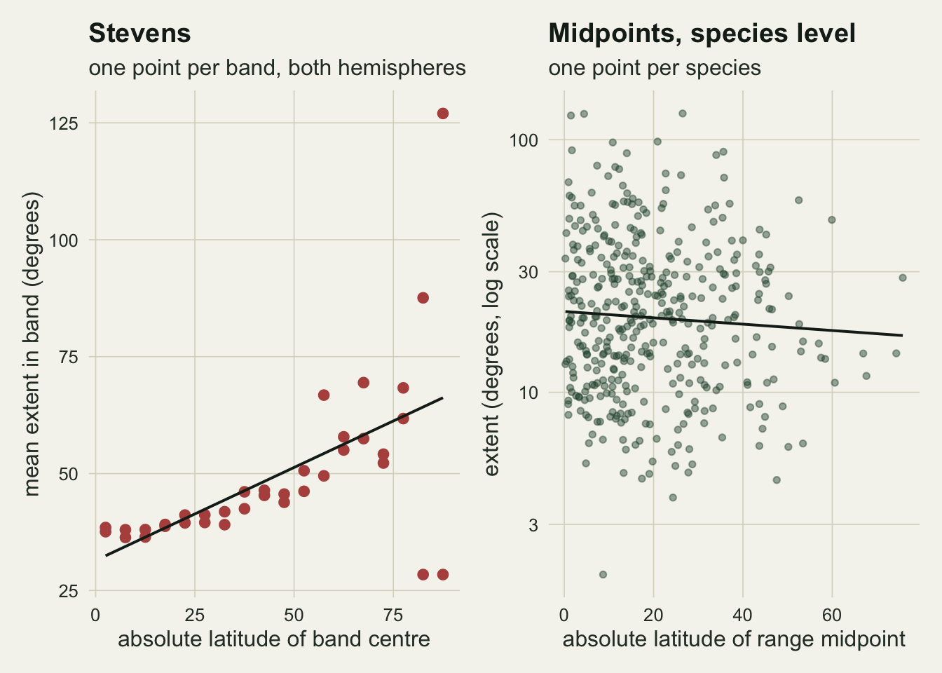
The left panel shows where the slope comes from. The busiest band holds 149 species, and the tropical band means sit close together. The emptiest band beyond 60 degrees holds 1, and a species with its midpoint in the tropics reaches such a band only if its range is long, so the mean there is a mean of the longest ranges in the world. The four outermost bands scatter widely above and below the line, because a band reached by 2 species or fewer takes their extents as its mean.
Stevens’ method finds a rule that is not there
n_world <- 500                          # worlds per cell, fixed before any rate was read
rate_cell <- function(peak_sd, ext_med, rule, edges = c(-90, 90), n = n_world) {
  cen <- band_centres(edges)
  r <- vapply(seq_len(n), function(i) both_methods(make_world(peak_sd, ext_med, rule, edges), cen),
              numeric(6))
  sig <- r[c("st.p", "mp.p", "rh.p"), ] < alpha_lev
  c(st_pos = mean(sig[1, ] & r["st.b", ] > 0), st_neg = mean(sig[1, ] & r["st.b", ] < 0),
    mp_pos = mean(sig[2, ] & r["mp.b", ] > 0), mp_neg = mean(sig[2, ] & r["mp.b", ] < 0),
    rh_pos = mean(sig[3, ] & r["rh.b", ] > 0), rh_neg = mean(sig[3, ] & r["rh.b", ] < 0))
}
peaks <- c(15, 25, 40, Inf); meds <- c(5, 10, 20, 40)
set.seed(1993)
sweep0 <- do.call(rbind, lapply(peaks, function(pk) do.call(rbind, lapply(meds, function(md)
  data.frame(peak_sd = pk, ext_med = md, t(rate_cell(pk, md, 0)))))))
sw <- function(pk, md, col) sweep0[sweep0$peak_sd == pk & sweep0$ext_med == md, col]
mcse_lo <- sqrt(0.025 * 0.975 / n_world); mcse_hi <- sqrt(0.25 / n_world)
print(sweep0)
peak_sd ext_med st_pos st_neg mp_pos mp_neg rh_pos rh_neg
1 15 5 0.300 0.120 0.024 0.028 0.032 0.108
2 15 10 0.852 0.000 0.016 0.020 0.042 0.118
3 15 20 1.000 0.000 0.022 0.036 0.026 0.160
4 15 40 1.000 0.000 0.000 0.178 0.010 0.274
5 25 5 0.188 0.226 0.018 0.030 0.026 0.096
6 25 10 0.478 0.096 0.020 0.020 0.008 0.104
7 25 20 0.968 0.000 0.010 0.040 0.002 0.196
8 25 40 1.000 0.000 0.000 0.284 0.000 0.848
9 40 5 0.100 0.272 0.016 0.038 0.010 0.104
10 40 10 0.180 0.282 0.006 0.036 0.000 0.216
11 40 20 0.538 0.060 0.000 0.154 0.000 0.742
12 40 40 0.998 0.000 0.000 0.816 0.000 1.000
13 Inf 5 0.048 0.378 0.002 0.092 0.002 0.090
14 Inf 10 0.012 0.732 0.000 0.192 0.000 0.238
15 Inf 20 0.000 0.992 0.000 0.690 0.000 0.928
16 Inf 40 0.000 1.000 0.000 1.000 0.000 1.000One world is an anecdote. The sweep above runs 500 worlds in each of sixteen cells, four widths of the richness peak by four median extents, all with no rule, and counts significant slopes of each sign at a nominal two sided five per cent. The number of worlds was fixed before any rate was read; the Monte Carlo standard error is 0.007 for a rate near the nominal 2.5 per cent per sign and at most 0.022 anywhere.
With a peak standard deviation of 25 degrees and a median extent of 20 degrees, Stevens’ method finds a significant positive rule in 96.8 per cent of worlds that have none. The midpoint regression in the same worlds is significant positive in 1.0 per cent and negative in 4.0 per cent.
The rate is not a property of the method alone. At a median extent of 5 degrees and the same peak, Stevens’ positive rate is 18.8 per cent and its negative rate 22.6 per cent: with short ranges few species reach far from their midpoints, the outer bands hold a few species each, and the test is wrong in both directions. At 10 degrees the positive rate is 47.8 per cent, and at 40 degrees it is 100.0 per cent. A narrower peak makes it worse (85.2 per cent at a peak of 15 degrees and extents of 10), a wider one milder (53.8 per cent at a peak of 40 and extents of 20). There is no single false positive rate for Stevens’ method to quote, only a surface over the peak width and the range size, and it runs to one wherever ranges are long compared with the peak.
Rohde’s band form, in the same sixteen cells, has its own error in the other direction. With a peak of 25 degrees and extents of 20 it is significant negative in 19.6 per cent of worlds and positive in 0.2 per cent; with a peak of 40 and extents of 20 the negative rate is 74.2 per cent. Its outer bands hold few species, so their means are noisy and, with a right-skewed extent distribution, tend to fall below the overall mean, and an unweighted regression gives those bands the same weight as the tropical ones. The species-level regression stays within two points of the nominal rate per sign in that cell, which is one reason it carries the rest of the post.
With no richness gradient the sign flips. Uniform midpoints put as many species near the poles as near the equator, the poles cut their ranges, and the high latitude band means fill with truncated extents. Stevens’ method is then significant negative in 99.2 per cent of worlds at a median extent of 20 degrees. The midpoint regression is not protected: it is significant negative in 9.2 per cent of worlds at 5 degrees, 19.2 per cent at 10, 69.0 per cent at 20 and 100.0 per cent at 40. The same clipping reaches the peaked worlds once ranges are long: at 40 degrees the midpoint method is significant negative in 28.4 per cent of worlds with a peak of 25 and 81.6 per cent with a peak of 40. Counting each species once removes the band sharing. It does nothing about the edge.
pk_lab <- c("15" = "peak sd 15", "25" = "peak sd 25", "40" = "peak sd 40", "Inf" = "flat (uniform)")
long0 <- rbind(
  data.frame(sweep0[, 1:2], method = "Stevens band means", sign = "positive", rate = sweep0$st_pos),
  data.frame(sweep0[, 1:2], method = "Stevens band means", sign = "negative", rate = sweep0$st_neg),
  data.frame(sweep0[, 1:2], method = "species midpoints", sign = "positive", rate = sweep0$mp_pos),
  data.frame(sweep0[, 1:2], method = "species midpoints", sign = "negative", rate = sweep0$mp_neg))
long0$peak <- factor(pk_lab[as.character(long0$peak_sd)], levels = pk_lab)
long0$sign <- factor(long0$sign, levels = c("positive", "negative"))
ggplot(long0, aes(ext_med, rate, colour = peak, linetype = sign)) +
  geom_hline(yintercept = alpha_lev / 2, colour = te_body, linewidth = 0.4, linetype = "dotted") +
  geom_line(linewidth = 0.8) + geom_point(size = 1.8) +
  facet_wrap(~ method) +
  scale_x_log10(breaks = meds) +
  scale_colour_manual(values = c(te_rust, te_gold, te_forest, te_ink), name = NULL) +
  scale_linetype_manual(values = c("solid", "dashed"), name = "significant slope") +
  labs(x = "median range extent (degrees, log scale)", y = "share of worlds",
       title = "No rule in any world, and how often one is found",
       subtitle = "dotted line: 2.5 per cent, the nominal rate for each sign") +
  guides(colour = guide_legend(nrow = 2), linetype = guide_legend(nrow = 2)) +
  theme_datasheet() + theme(legend.position = "bottom")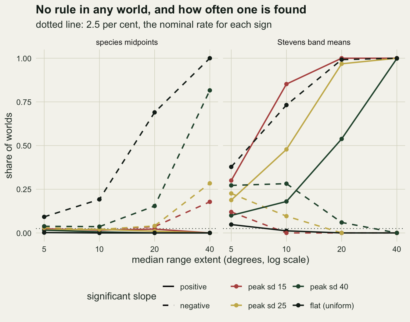
A real rule, read backwards
A method that invents a rule may still find a real one. The next sweep fixes the median extent at 20 degrees and gives every world a true slope of 0.5 or of -0.5.
set.seed(1994)
rules <- do.call(rbind, lapply(peaks, function(pk) do.call(rbind, lapply(c(-0.5, 0.5), function(rl)
  data.frame(peak_sd = pk, rule = rl, t(rate_cell(pk, 20, rl)))))))
ru <- function(pk, rl, col) rules[rules$peak_sd == pk & rules$rule == rl, col]
print(rules)
peak_sd rule st_pos st_neg mp_pos mp_neg rh_pos rh_neg
1 15 -0.5 0.998 0.000 0.000 0.856 0.000 0.660
2 15 0.5 1.000 0.000 0.738 0.000 0.304 0.002
3 25 -0.5 0.632 0.070 0.000 0.998 0.000 0.936
4 25 0.5 1.000 0.000 0.974 0.000 0.354 0.000
5 40 -0.5 0.086 0.666 0.000 1.000 0.000 1.000
6 40 0.5 1.000 0.000 0.988 0.000 0.006 0.010
7 Inf -0.5 0.000 1.000 0.000 1.000 0.000 1.000
8 Inf 0.5 0.036 0.650 0.698 0.000 0.000 0.094With a true negative rule, ranges shrinking towards the poles, and a peak of 25 degrees, Stevens’ method is significant positive in 63.2 per cent of worlds and significant negative, the right answer, in 7.0 per cent. With a peak of 15 degrees the wrong sign comes out in 99.8 per cent. The geometry of the peak outweighs a real rule of this size. The midpoint method finds the negative rule in 99.8 per cent of worlds at a peak of 25.
A positive rule with uniform midpoints turns the problem over. Clipping now works against the rule: the longest ranges sit near the poles and are the ones cut. Stevens’ method is significant negative in 65.0 per cent of those worlds, the reverse of the truth, and the midpoint method detects the positive rule in 69.8 per cent. With a narrow peak of 15 degrees the midpoint method also loses power, 73.8 per cent, because few species have midpoints at high latitude to carry the slope. Rohde’s band form is weaker still against the positive rule: 35.4 per cent at a peak of 25 and 0.0 per cent with uniform midpoints, against 93.6 per cent for the negative rule at a peak of 25.
rl <- rbind(
  data.frame(rules[, 1:2], method = "Stevens band means",
             right = ifelse(rules$rule > 0, rules$st_pos, rules$st_neg),
             wrong = ifelse(rules$rule > 0, rules$st_neg, rules$st_pos)),
  data.frame(rules[, 1:2], method = "species midpoints",
             right = ifelse(rules$rule > 0, rules$mp_pos, rules$mp_neg),
             wrong = ifelse(rules$rule > 0, rules$mp_neg, rules$mp_pos)))
rl$peak <- factor(pk_lab[as.character(rl$peak_sd)], levels = pk_lab)
rl$truth <- factor(ifelse(rl$rule > 0, "true rule: extent grows polewards",
                          "true rule: extent shrinks polewards"),
                   levels = c("true rule: extent grows polewards", "true rule: extent shrinks polewards"))
ggplot(rl, aes(peak, fill = method)) +
  geom_col(aes(y = right), position = position_dodge(width = 0.75), width = 0.7) +
  geom_col(aes(y = -wrong), position = position_dodge(width = 0.75), width = 0.7, alpha = 0.55) +
  geom_hline(yintercept = 0, colour = te_ink, linewidth = 0.4) +
  facet_wrap(~ truth, ncol = 1) +
  scale_fill_manual(values = c(te_rust, te_forest), name = NULL) +
  scale_y_continuous(limits = c(-1, 1), breaks = c(-1, -0.5, 0, 0.5, 1),
                     labels = c("1", "0.5", "0", "0.5", "1")) +
  labs(x = "distribution of range midpoints", y = "share of worlds",
       title = "A real rule, found with the right or the wrong sign",
       subtitle = "above zero: significant with the true sign; below: significant with the opposite sign") +
  theme_datasheet() + theme(legend.position = "bottom")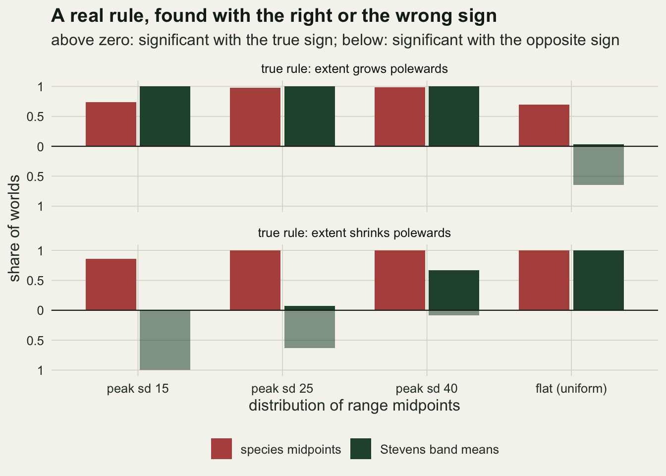
Four ways to treat a clipped range
Two cells from the sweeps are worth repairing: an equatorial peak of 25 degrees, where band sharing is the problem, and uniform midpoints, where the edge is. Both with a median extent of 20 degrees and each of the three true slopes. Four treatments are compared with the plain tests.
The first two act on the midpoint regression directly. Dropping every species whose range touches a pole is a common repair. Censored regression keeps those species and treats their observed log extent as a lower bound, with survreg from the survival package. The other two are null distributions for either statistic. The midpoint shuffle keeps each species’ observed extent, gives it the midpoint of another species and clips again at the poles, which is the permutation with extents fixed. The re-clipped null goes one step further back: it fits a censored lognormal to the extents with no latitude term, draws new extents from it, places them at resampled midpoints and clips them, so the null world goes through the same edge as the data. That second null is a parametric bootstrap written for this post in the spirit of Colwell and Hurtt’s geometric null models, not a published named test.
n_edge <- 200; n_perm <- 99             # worlds per cell and null draws, fixed in advance
# slopes of log extent on absolute midpoint for many worlds at once (columns)
slope_cols <- function(lo, hi) {
  x <- abs((lo + hi) / 2); y <- log(hi - lo)
  xc <- x - rep(colMeans(x), each = nrow(x))
  colSums(xc * y) / colSums(xc^2)
}
treat <- function(w, cen = band_centres(w$edges)) {
  ed <- w$edges; half <- w$ext / 2; inner <- !w$touch
  st <- stevens_means(w$lo, w$hi, w$ext, cen)
  obs_st <- slope_test(st$lat, st$mean_ext); obs_mp <- slope_test(abs(w$mid), log(w$ext))
  ex <- slope_test(abs(w$mid[inner]), log(w$ext[inner]))
  cz <- summary(survreg(Surv(log(w$ext), inner) ~ abs(w$mid), dist = "gaussian"))$table[2, c(1, 4)]
  fit0 <- survreg(Surv(log(w$ext), inner) ~ 1, dist = "gaussian")
  # null 1: shuffle midpoints among species, keep each observed extent, clip again
  mm <- vapply(seq_len(n_perm), function(i) sample(w$mid), numeric(n_sp))
  lo1 <- pmax(mm - half, ed[1]); hi1 <- pmin(mm + half, ed[2])
  # null 2: extents drawn from a censored lognormal fit, midpoints resampled, clipped again
  mm2 <- matrix(sample(w$mid, n_sp * n_perm, replace = TRUE), n_sp)
  ee2 <- matrix(exp(rnorm(n_sp * n_perm, coef(fit0), fit0$scale)), n_sp)
  lo2 <- pmax(mm2 - ee2 / 2, ed[1]); hi2 <- pmin(mm2 + ee2 / 2, ed[2])
  st_null <- function(lo, hi) vapply(seq_len(n_perm), function(i) {
    s <- stevens_means(lo[, i], hi[, i], hi[, i] - lo[, i], cen)
    slope_test(s$lat, s$mean_ext)[["b"]]
  }, numeric(1))
  # two-sided test around the centre of the null, sign relative to that centre
  call_it <- function(nb, ob) {
    p <- (1 + sum(abs(nb - mean(nb)) >= abs(ob - mean(nb)))) / (n_perm + 1)
    sign(ob - mean(nb)) * (p < alpha_lev)
  }
  sig_ols <- function(bp) sign(bp[[1]]) * (bp[[2]] < alpha_lev)
  c(st_ols = sig_ols(obs_st), mp_ols = sig_ols(obs_mp), mp_excl = sig_ols(ex), mp_cens = sig_ols(cz),
    st_shuffle = call_it(st_null(lo1, hi1), obs_st[["b"]]),
    mp_shuffle = call_it(slope_cols(lo1, hi1), obs_mp[["b"]]),
    st_reclip = call_it(st_null(lo2, hi2), obs_st[["b"]]),
    mp_reclip = call_it(slope_cols(lo2, hi2), obs_mp[["b"]]),
    touch = mean(w$touch), n_inner = sum(inner),
    lat_inner = mean(abs(w$mid[inner])), lat_all = mean(abs(w$mid)))
}
set.seed(1998)
edge_cells <- expand.grid(peak_sd = c(25, Inf), rule = c(0, -0.5, 0.5))
edge_res <- lapply(seq_len(nrow(edge_cells)), function(j)
  replicate(n_edge, treat(make_world(edge_cells$peak_sd[j], 20, edge_cells$rule[j]))))
meth <- c("st_ols", "mp_ols", "mp_excl", "mp_cens", "st_shuffle", "mp_shuffle", "st_reclip", "mp_reclip")
edge_tab <- do.call(rbind, lapply(seq_len(nrow(edge_cells)), function(j) {
  r <- edge_res[[j]]
  data.frame(peak_sd = edge_cells$peak_sd[j], rule = edge_cells$rule[j], method = meth,
             pos = rowMeans(r[meth, ] > 0), neg = rowMeans(r[meth, ] < 0),
             touch = mean(r["touch", ]), row.names = NULL)
}))
eg <- function(pk, rl, m, sgn) edge_tab[edge_tab$peak_sd == pk & edge_tab$rule == rl & edge_tab$method == m, sgn]
sel <- rowMeans(edge_res[[2]][c("touch", "n_inner", "lat_inner", "lat_all"), ])
pk_max <- max(unlist(edge_tab[edge_tab$peak_sd == 25 & edge_tab$rule == 0 & grepl("^mp", edge_tab$method), c("pos", "neg")]))
mcse_edge_lo <- sqrt(0.025 * 0.975 / n_edge)
print(edge_tab)
peak_sd rule method pos neg touch
1 25 0.0 st_ols 0.965 0.000 0.0070375
2 25 0.0 mp_ols 0.020 0.045 0.0070375
3 25 0.0 mp_excl 0.010 0.055 0.0070375
4 25 0.0 mp_cens 0.035 0.040 0.0070375
5 25 0.0 st_shuffle 0.100 0.030 0.0070375
6 25 0.0 mp_shuffle 0.020 0.025 0.0070375
7 25 0.0 st_reclip 0.020 0.015 0.0070375
8 25 0.0 mp_reclip 0.030 0.020 0.0070375
9 Inf 0.0 st_ols 0.000 0.995 0.1408875
10 Inf 0.0 mp_ols 0.000 0.640 0.1408875
11 Inf 0.0 mp_excl 0.000 0.835 0.1408875
12 Inf 0.0 mp_cens 0.200 0.000 0.1408875
13 Inf 0.0 st_shuffle 0.000 0.090 0.1408875
14 Inf 0.0 mp_shuffle 0.000 0.165 0.1408875
15 Inf 0.0 st_reclip 0.010 0.005 0.1408875
16 Inf 0.0 mp_reclip 0.000 0.040 0.1408875
17 25 -0.5 st_ols 0.665 0.050 0.0019125
18 25 -0.5 mp_ols 0.000 0.990 0.0019125
19 25 -0.5 mp_excl 0.000 0.990 0.0019125
20 25 -0.5 mp_cens 0.000 0.990 0.0019125
21 25 -0.5 st_shuffle 0.195 0.145 0.0019125
22 25 -0.5 mp_shuffle 0.000 0.985 0.0019125
23 25 -0.5 st_reclip 0.110 0.035 0.0019125
24 25 -0.5 mp_reclip 0.000 0.985 0.0019125
25 Inf -0.5 st_ols 0.000 1.000 0.0571750
26 Inf -0.5 mp_ols 0.000 1.000 0.0571750
27 Inf -0.5 mp_excl 0.000 1.000 0.0571750
28 Inf -0.5 mp_cens 0.000 1.000 0.0571750
29 Inf -0.5 st_shuffle 0.000 0.965 0.0571750
30 Inf -0.5 mp_shuffle 0.000 1.000 0.0571750
31 Inf -0.5 st_reclip 0.000 0.890 0.0571750
32 Inf -0.5 mp_reclip 0.000 1.000 0.0571750
33 25 0.5 st_ols 1.000 0.000 0.0257875
34 25 0.5 mp_ols 0.985 0.000 0.0257875
35 25 0.5 mp_excl 0.880 0.000 0.0257875
36 25 0.5 mp_cens 1.000 0.000 0.0257875
37 25 0.5 st_shuffle 0.005 0.000 0.0257875
38 25 0.5 mp_shuffle 0.995 0.000 0.0257875
39 25 0.5 st_reclip 0.000 0.040 0.0257875
40 25 0.5 mp_reclip 0.990 0.000 0.0257875
41 Inf 0.5 st_ols 0.015 0.645 0.2684250
42 Inf 0.5 mp_ols 0.710 0.000 0.2684250
43 Inf 0.5 mp_excl 0.430 0.000 0.2684250
44 Inf 0.5 mp_cens 1.000 0.000 0.2684250
45 Inf 0.5 st_shuffle 0.205 0.000 0.2684250
46 Inf 0.5 mp_shuffle 1.000 0.000 0.2684250
47 Inf 0.5 st_reclip 0.015 0.000 0.2684250
48 Inf 0.5 mp_reclip 1.000 0.000 0.2684250Each null uses 99 draws, the p value is two sided around the centre of the null, and each cell has 200 worlds, a Monte Carlo standard error of 0.011 near the nominal rate per sign.
With uniform midpoints and no rule, 14.1 per cent of species touch a pole. Dropping them makes the midpoint method worse, not better: significant negative in 83.5 per cent of worlds against 64.0 per cent for the plain regression. The selection is the reason. A species with its midpoint at absolute latitude m can stay clear of the pole only if its extent is below twice the distance 90 minus m, so the ranges that survive the filter are capped more tightly the closer they sit to a pole, and the filter builds the negative slope back in by selection rather than by truncation. It also thins the high latitudes: the mean absolute midpoint of the 344 species left is 39.1 degrees against 44.1 for all species. With a true positive rule the filter keeps 43.0 per cent power against 71.0 per cent for the plain test.
Censored regression overcorrects. With no rule it is significant positive in 20.0 per cent of uniform worlds. The censoring is not of the kind survreg assumes. A clipped extent is the distance from the inner limit to the pole, which itself grows with the true extent, so the lower bound carries information the model ignores.
The midpoint shuffle shrinks the rate of spurious negative slopes to 16.5 per cent and keeps power: 100.0 per cent against the positive rule. It stays above nominal because the observed extents it moves are already clipped: a range cut at the pole and moved to the tropics is not given back the length it lost, so the null carries less of the edge than the data. The re-clipped null is the only midpoint treatment close to nominal in both geometries: 0.0 and 4.0 per cent positive and negative with uniform midpoints, 3.0 and 2.0 per cent with the peak, and 100.0 per cent power against the positive rule that the plain midpoint test finds in 71.0 per cent of worlds.
Stevens’ statistic can be sized the same way, and that is where its problem shows. Against the re-clipped null it rejects a true null in 3.5 per cent of peaked worlds, both signs together against a nominal five, but against a true positive rule in the same worlds it is significant positive in 0.0 per cent. Once the null carries the geometry, the band means have little left to say about a positive rule. With the peak and a true negative rule they are significant with the wrong sign in 11.0 per cent of worlds and with the right one in 3.5 per cent; only with uniform midpoints do they find the negative rule, in 89.0 per cent of worlds, where the midpoint tests find it in all of them. The midpoint shuffle gives Stevens’ statistic 10.0 per cent false positives with the peak and 0.5 per cent power against the positive rule. With a peak of 25 degrees clipping touches 0.7 per cent of species, and no midpoint treatment is significant with either sign in more than 5.5 per cent of worlds with no rule.
m_lab <- c(st_ols = "Stevens, OLS test", st_shuffle = "Stevens, midpoint shuffle",
           st_reclip = "Stevens, re-clipped null", mp_ols = "midpoints, OLS",
           mp_excl = "midpoints, edge species dropped", mp_cens = "midpoints, censored regression",
           mp_shuffle = "midpoints, midpoint shuffle", mp_reclip = "midpoints, re-clipped null")
el <- rbind(data.frame(edge_tab[, 1:3], sign = "positive", rate = edge_tab$pos),
            data.frame(edge_tab[, 1:3], sign = "negative", rate = edge_tab$neg))
el$method <- factor(m_lab[el$method], levels = rev(m_lab))
el$geom <- factor(ifelse(is.infinite(el$peak_sd), "flat midpoints", "equator peak (sd 25)"),
                  levels = c("equator peak (sd 25)", "flat midpoints"))
tr_lab <- c("0" = "no rule", "-0.5" = "true slope -0.5", "0.5" = "true slope +0.5")
el$truth <- factor(tr_lab[as.character(el$rule)], levels = tr_lab)
el$sign <- factor(el$sign, levels = c("positive", "negative"))
ggplot(el, aes(rate, method, colour = sign, shape = sign)) +
  geom_vline(xintercept = alpha_lev / 2, colour = te_body, linetype = "dotted", linewidth = 0.4) +
  geom_point(size = 2.4, stroke = 0.9) +
  facet_grid(truth ~ geom) +
  scale_colour_manual(values = c(te_forest, te_rust), name = "significant slope") +
  scale_shape_manual(values = c(16, 17), name = "significant slope") +
  scale_x_continuous(limits = c(0, 1), breaks = c(0, 0.5, 1)) +
  labs(x = "share of worlds", y = NULL, title = "Eight ways to test for the rule",
       subtitle = "dotted line: 2.5 per cent per sign") +
  theme_datasheet() + theme(legend.position = "bottom", panel.spacing = unit(1, "lines"))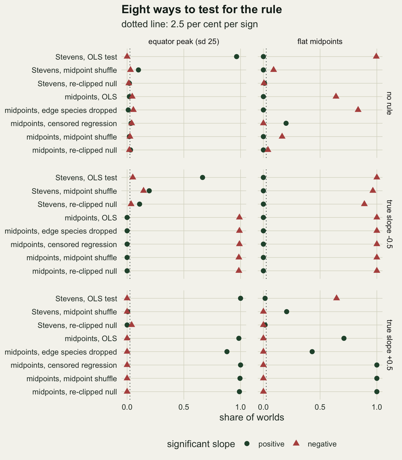
Continents, hemispheres and body size
Real data rarely run from pole to pole. The first variant puts the hard edges at 55 degrees south and 72 degrees north, roughly the limits of land in the Americas, and keeps absolute latitude as the axis. The second is the hemisphere-only data set, northern species only, with the equator treated as the southern edge of the domain.
set.seed(2004)
cont <- rbind(peak = rate_cell(25, 20, 0, edges = c(-55, 72)),
              flat = rate_cell(Inf, 20, 0, edges = c(-55, 72)))
# hemisphere only: equator treated as a hard edge, northern species only
hemi_world <- function(peak_sd, ext_med) {
  m <- abs(draw_mid(n_sp, peak_sd, c(-90, 90)))
  ext <- ext_med * exp(rnorm(n_sp, 0, sd_log))
  lo <- pmax(m - ext / 2, 0); hi <- pmin(m + ext / 2, 90)
  list(lo = lo, hi = hi, ext = hi - lo, mid = (lo + hi) / 2, edges = c(0, 90),
       touch = lo <= 0 | hi >= 90)
}
hemi <- vapply(seq_len(n_world), function(i) both_methods(hemi_world(25, 20)), numeric(6))
hemi_rates <- c(st_pos = mean(hemi["st.p", ] < alpha_lev & hemi["st.b", ] > 0),
                mp_pos = mean(hemi["mp.p", ] < alpha_lev & hemi["mp.b", ] > 0),
                mp_neg = mean(hemi["mp.p", ] < alpha_lev & hemi["mp.b", ] < 0))
print(cont); print(hemi_rates)
st_pos st_neg mp_pos mp_neg rh_pos rh_neg
peak 0.976 0.00 0 0.258 0 0.822
flat 0.000 0.99 0 0.936 0 0.970st_pos mp_pos mp_neg
0.996 1.000 0.000 With continental limits and a peak of 25 degrees, Stevens’ method is significant positive in 97.6 per cent of worlds with no rule and the midpoint method significant negative in 25.8 per cent, against 4.0 per cent in the pole to pole world. With uniform midpoints the midpoint method is significant negative in 93.6 per cent. A shorter domain puts both edges closer to the richness peak, and the southern limit at 55 degrees is an edge at a latitude where the pole to pole world had none.
The hemisphere-only design is the worst of all. Cutting the domain at the equator clips the ranges of every species that crosses it, and those are the tropical species. Stevens’ method is significant positive in 99.6 per cent of worlds with no rule and the midpoint method in 100.0 per cent. Here the midpoint method manufactures the rule too, from the edge alone. The equator is not a boundary of anything a species does, and a data set that stops there must keep the southern limits of the ranges that cross it.
The same band sharing drives the assemblage version of Bergmann’s rule, in which body size is averaged over the species present in each grid cell or band and the means are regressed on latitude. The chunk below gives every species a lognormal body size drawn independently of its range and of everything else, and averages it over bands with the same machinery.
# assemblage Bergmann: body size unrelated to anything, averaged per band
berg <- vapply(seq_len(n_world), function(i) {
  w <- make_world(25, 20, 0); size <- rlnorm(n_sp, 3, 1)
  s <- stevens_means(w$lo, w$hi, size, band_centres(w$edges))
  c(band = slope_test(s$lat, log(s$mean_ext))[["p"]], sp = slope_test(abs(w$mid), log(size))[["p"]])
}, numeric(2))
berg_rates <- rowMeans(berg < alpha_lev)
berg_rates
band sp
0.576 0.048 The band-level regression of the log of mean body size on absolute latitude is significant in 57.6 per cent of worlds; the species-level regression of log body size on absolute midpoint in 4.8 per cent. There is no geometry in body size, so the excess comes from how the band means are built: neighbouring bands average mostly the same species, which makes the means a smooth, autocorrelated series with far fewer independent values than bands, and the outermost bands average only a few species each. That is the same lesson as the family bootstrap in Checking a macroecological pattern, with space in place of phylogeny.
What to report
Report species-level results, with one point per species, before any band or cell means. If band means are shown as a figure, Stevens’ or Rohde’s, do not attach a regression test to them. Stevens’ bands share species, and the test was wrong in these worlds whether or not a rule existed. Rohde’s midpoint bands share none, but the outer ones rest on a few species each: that test gave a false negative rule in 19.6 per cent of worlds with no rule and a peak of 25, and found the positive rule in 35.4 per cent.
Say where the domain ends and how many species have a range limit on that edge. At a median extent of 20 degrees and a flat richness distribution the share was 14.1 per cent, and that was enough to turn the midpoint method significant in most worlds with no rule. A reader cannot judge a range size gradient without that number.
Do not drop edge-touching species and call the remainder clean. The filter is a selection on range size that depends on latitude, and in the flat worlds above it made the false rule more frequent.
Test the slope against a null that goes through the same edge as the data. The re-clipped null here is one way to do it, and the midpoint shuffle is a cheaper approximation that stays liberal when clipping is common. Give the null’s centre next to the observed slope, because under a hard edge the expected slope with no rule is not zero.
If the data set is one hemisphere, say what was done with the ranges that cross the equator. Treating the equator as an edge produced the rule in essentially every world here.
Honest limits
The domain has one dimension. Range extent here is a length on the latitude axis, which is how Stevens and Rohde measured it, but it ignores longitude, the shape of continents and the way land area narrows towards the poles. Colwell and Hurtt’s models were one-dimensional too; two-dimensional versions that add continent shape can move the rates above. These numbers belong to a line with two ends, not to a map.
The worlds are simple in ways real faunas are not. Extents are lognormal with a fixed spread of 0.7 on the log scale, species are independent of each other, and a rule is a straight slope in log extent on absolute latitude, the same in both hemispheres. There is no phylogeny, so the dependence that Checking a macroecological pattern deals with is absent, and a real analysis has both kinds at once.
Rohde’s band form is reported only for the first two sweeps, as an unweighted regression of band mean extent on band latitude. The edge treatments, and a regression weighted by the number of species per band, were not applied to it, so its rates above belong to that one form.
The re-clipped null is a parametric bootstrap under one generating model: lognormal extents independent of latitude, midpoints resampled from the observed ones. It is close to nominal here partly because the data were generated from the same family. With a skewed extent distribution that the censored lognormal fits badly, or with midpoints that were themselves shifted by clipping, it will drift, and nothing above measures how far.
The sweeps set the median extent and the width of the richness peak by hand, and the rejection rates move a long way across them. None of the numbers is a rate to quote for a real taxon; the point is that the answer depends on both, so a study should report both.
Every test uses a nominal five per cent split into two signs, and every rate counts a significant slope of the stated sign. A Stevens slope that is significant but small in absolute terms counts the same as a large one. The effect size of the false rule, in degrees of extent per degree of latitude, is not measured here.
References
Stevens GC 1989 American Naturalist 133(2):240-256 (10.1086/284913)
Rohde K, Heap M, Heap D 1993 American Naturalist 142(1):1-16 (10.1086/285526)
Colwell RK, Hurtt GC 1994 American Naturalist 144(4):570-595 (10.1086/285695)
Gaston KJ, Blackburn TM, Spicer JI 1998 Trends in Ecology and Evolution 13(2):70-74 (10.1016/S0169-5347(97)01236-6)
Peres-Neto PR, Dray S, ter Braak CJF 2017 Ecography 40(7):806-816 (10.1111/ecog.02302)