fc <- function(L, e, t) {
  P <- L / sum(L); wi <- rowSums(P); wj <- colSums(P)
  es <- e - sum(wi * e); es <- es / sqrt(sum(wi * es^2))     # weighted standardisation
  ts <- t - sum(wj * t); ts <- ts / sqrt(sum(wj * ts^2))
  sum(P * outer(es, ts))
}Checking a trait environment analysis
R
traits
functional ecology
community ecology
model diagnostics
ecology tutorial
A fourth corner correlation can come back highly significant when the true trait to environment link is exactly zero. The permutation null you pick decides it.
Corrected 14 October 2026: the niche width section called the widest niches the one place the site shuffle behaves; its rate there is still above the nominal level, so it now says the shuffle comes closest to that level there, and that the plots hold nearly, not exactly, the same proportions. The advice on reading a single reported p-value said the missing half is the half that fails; it now says this is usually so when the true link is zero.
Corrected 7 October 2026: the advice on reporting the statistic said a correlation of the size seen on null data is worth nothing whatever any test says; the max test the post recommends keeps its level, so it now says such a size is no evidence of a link on its own or with a single shuffle behind it.
Corrected 30 September 2026: the post gave the product of the two rejection rates as the expected rate at which both shuffles reject together; the two tests judge the same statistic and are not independent, so it now calls the product a rough guide.
You have a trait, an environmental variable, and an abundance table. You compute a community weighted mean correlation or the fourth corner statistic, and it comes back small but significant. This post builds a data set where the true link between the trait and the environment is exactly zero, gets a significant p-value out of it, and then measures how often that happens.
The short version: that p-value came from a null hypothesis that is not the one you wanted tested, and there is a second null available, on the same statistic and the same data, that says there is nothing there.
Two nulls, and neither of them is yours
The fourth corner correlation is an abundance weighted correlation between the site environment and the species trait, taken over the whole table at once:
It has no parametric distribution worth trusting, so it gets a permutation test. There are two obvious things to shuffle, and they are not equivalent.
Shuffling the rows of the abundance table moves whole communities between sites. It breaks the link between the environment and the species composition, and it leaves the link between the species and their traits alone. Shuffling the columns moves whole species between trait values. It breaks the trait link and leaves the environment link alone. In the fourth corner literature these are permutation models 2 and 4, and each has its own null hypothesis: model 2 says the environment does not affect where the species are, model 4 says the traits do not affect where the species are.
Neither of those is the hypothesis in your paper. Yours is that the trait has nothing to do with the environment, and that is true whenever either of the two links is missing. That is the whole problem in one sentence, and the rest of this post is what it costs.
sim <- function(seed, env_drives, trait_drives, n_site = 30, n_sp = 25, tol = 0.25) {
  set.seed(seed)
  e <- runif(n_site)                                  # the environment you measured
  g <- if (env_drives) e else runif(n_site)           # the gradient the species actually track
  o <- runif(n_sp, -0.1, 1.1)                         # species optima on that gradient
  t <- if (trait_drives) 12 * o + rnorm(n_sp, 0, 1.5) else rnorm(n_sp, 6, 4)
  mu <- outer(g, o, function(x, y) exp(-(x - y)^2 / (2 * tol^2)))
  L  <- matrix(rpois(n_site * n_sp, sweep(mu, 2, rlnorm(n_sp, log(20), 0.4), "*")), n_site, n_sp)
  ok_i <- rowSums(L) > 0; ok_j <- colSums(L) > 0
  list(L = L[ok_i, ok_j, drop = FALSE], e = e[ok_i], t = t[ok_j])
}
pv <- function(s, nperm = 199) {
  r0 <- fc(s$L, s$e, s$t)
  d2 <- replicate(nperm, fc(s$L[sample(nrow(s$L)), , drop = FALSE], s$e, s$t))   # shuffle sites
  d4 <- replicate(nperm, fc(s$L[, sample(ncol(s$L)), drop = FALSE], s$e, s$t))   # shuffle species
  c(r = r0, p_sites = (1 + sum(abs(d2) >= abs(r0))) / (nperm + 1),
    p_species = (1 + sum(abs(d4) >= abs(r0))) / (nperm + 1))
}
The two switches are independent. env_drives decides whether the variable you measured is the gradient the plants respond to. trait_drives decides whether the trait you measured predicts where a species sits on that gradient. The trait to environment link exists only when both are on.
The eighty per cent
Four hundred data sets per row, 199 permutations per test, nominal five per cent.
rate <- function(env_drives, trait_drives, nrep = 400, base = 0) {
  m <- t(vapply(seq_len(nrep), function(k)
    pv(sim(base + k, env_drives, trait_drives)), numeric(3)))
  c(mean_abs_r = mean(abs(m[, 1])), by_sites = mean(m[, 2] <= 0.05),
    by_species = mean(m[, 3] <= 0.05), max_test = mean(pmax(m[, 2], m[, 3]) <= 0.05))
}
tab <- rbind(
  "environment drives, trait random" = rate(TRUE,  FALSE, base = 3110000),
  "trait drives, environment random" = rate(FALSE, TRUE,  base = 3120000),
  "both (a real link)"               = rate(TRUE,  TRUE,  base = 3130000),
  "neither"                          = rate(FALSE, FALSE, base = 3140000))
print(round(tab, 3))
mean_abs_r by_sites by_species max_test
environment drives, trait random 0.117 0.805 0.045 0.045
trait drives, environment random 0.094 0.048 0.752 0.048
both (a real link) 0.642 1.000 1.000 1.000
neither 0.022 0.038 0.038 0.002Read the first two rows. In both of them the true trait to environment link is zero, so every rejection is a false positive. Shuffling sites rejects 80% of the time on the first row. Shuffling species rejects 75% of the time on the second. Each test is fine on the row where its own null is true and catastrophic on the row where it is not, and the two rows are mirror images because the two tests are mirror images.
The last column takes the larger of the two p-values, which is the same as demanding that both shuffles reject. It sits at 4.5% and 4.8% on the two null rows against a nominal 5, keeps 100% power on the row with a real link, and drops to 0.2% when nothing at all is going on. That last number is not a bug. With both component nulls true, both shuffles have to reject by chance at once. If the two tests were independent that would happen about 0.001 of the time; they are not, because both judge the same observed statistic, so the product is only a rough guide, and 0.002 is what came out. The max test is conservative exactly where being conservative costs nothing. This is ter Braak, Cormont & Dray (2012); with 400 replicates the Monte Carlo error on a five per cent rate is about 1.1 points, which is small next to the numbers in the first two rows.
Why the site shuffle is narrow
Take one data set from the first row and build both null distributions properly.
s  <- sim(3110001, env_drives = TRUE, trait_drives = FALSE)
r0 <- fc(s$L, s$e, s$t)
n_sites   <- replicate(1999, fc(s$L[sample(nrow(s$L)), , drop = FALSE], s$e, s$t))
n_species <- replicate(1999, fc(s$L[, sample(ncol(s$L)), drop = FALSE], s$e, s$t))
two <- c(observed = r0, sd_sites = sd(n_sites), sd_species = sd(n_species),
         width_ratio = sd(n_species) / sd(n_sites),
         p_sites = (1 + sum(abs(n_sites) >= abs(r0))) / 2000,
         p_species = (1 + sum(abs(n_species) >= abs(r0))) / 2000)
print(round(two, 4))
observed sd_sites sd_species width_ratio p_sites p_species
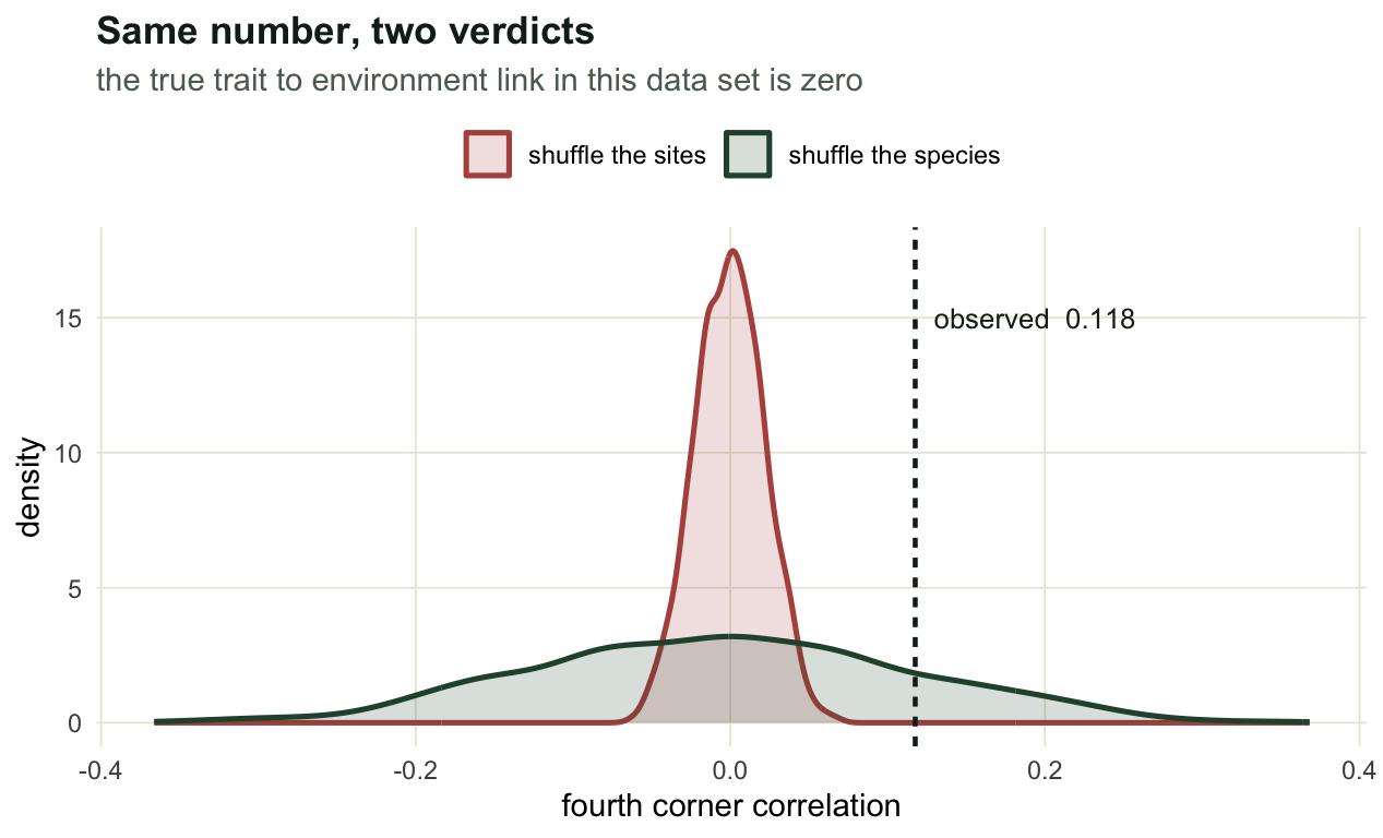
0.1175 0.0219 0.1208 5.5131 0.0005 0.3470 One statistic, one data set, 0.0005 against 0.347. The first of those is the smallest p-value 1999 permutations can produce, so the site shuffle is not merely rejecting, it is rejecting as hard as it is able to. The two nulls differ by a factor of 5.5 in width, and that factor is the entire disagreement.
Here is where the width comes from. Every species in this data set occupies a band of the gradient, so the community weighted mean trait at a site is an average over the handful of species that live near that site’s position. Neighbouring sites share species, so their weighted means are nearly the same number, and the series of weighted means is a smooth curve along the gradient. It is a random curve, because the trait values were dealt out at random, but a smooth one, and a smooth random curve has a large correlation with the gradient far more often than a set of independent draws does. Shuffling sites compares that curve against reorderings of itself, which are not smooth. The observed value is not extreme; the null it is being judged against is too narrow.
Shuffling species keeps the smoothness and reassigns the trait values, which is the comparison that actually contains the observed value.
More sites do not help
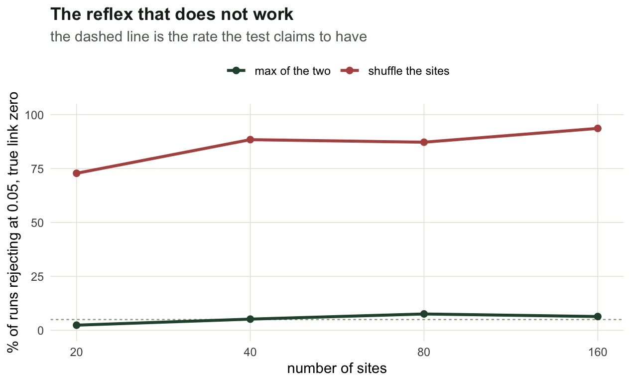
The usual reflex when a test misbehaves is to blame the sample size. Take the first row of the table and grow it.
grow <- t(vapply(c(20, 40, 80, 160), function(n) {
  m <- t(vapply(1:250, function(k) pv(sim(3170000 + k, TRUE, FALSE, n_site = n)), numeric(3)))
  c(n_site = n, mean_abs_r = mean(abs(m[, 1])), by_sites = mean(m[, 2] <= 0.05),
    max_test = mean(pmax(m[, 2], m[, 3]) <= 0.05))
}, numeric(4)))
print(round(grow, 3))
n_site mean_abs_r by_sites max_test
[1,] 20 0.105 0.728 0.024
[2,] 40 0.121 0.884 0.052
[3,] 80 0.111 0.872 0.076
[4,] 160 0.115 0.936 0.064The false positive rate goes from 73% at twenty sites to 94% at a hundred and sixty, while the statistic itself sits at the same 0.11 throughout. This is not a small sample problem and a field season will not fix it. Doubling the sites narrows the site shuffle null and leaves the smooth curve exactly as smooth as it was, so the gap between them widens. The max test stays between 2.4% and 7.6% across the same range.
It peaks where your data are interesting
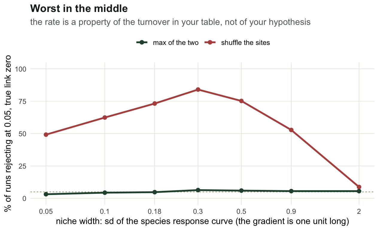
The smooth curve needs species that occupy bands. Widen every niche until each species is everywhere and the curve flattens; narrow them until each site holds one species and it stops being a curve. So the inflation should be worst in between, which is where field data live.
bray <- function(L) {
  R <- L / rowSums(L); n <- nrow(R); s <- 0; k <- 0
  for (i in 1:(n - 1)) for (j in (i + 1):n) { s <- s + sum(abs(R[i, ] - R[j, ])) / 2; k <- k + 1 }
  s / k
}
grid <- c(0.05, 0.10, 0.18, 0.30, 0.50, 0.90, 2.00)
br <- t(vapply(grid, function(tl) {
  m <- t(vapply(1:250, function(k) pv(sim(3150000 + k, TRUE, FALSE, tol = tl)), numeric(3)))
  c(niche_width = tl,
    turnover = mean(vapply(1:20, function(k) bray(sim(3160000 + k, TRUE, FALSE, tol = tl)$L), 0)),
    by_sites = mean(m[, 2] <= 0.05), max_test = mean(pmax(m[, 2], m[, 3]) <= 0.05))
}, numeric(4)))
print(round(br, 3))
niche_width turnover by_sites max_test
[1,] 0.05 0.850 0.492 0.032
[2,] 0.10 0.725 0.624 0.044
[3,] 0.18 0.558 0.732 0.048
[4,] 0.30 0.376 0.840 0.064
[5,] 0.50 0.219 0.752 0.060
[6,] 0.90 0.139 0.528 0.056
[7,] 2.00 0.118 0.088 0.056The rate is a hump. It tops out at 84% around a mean Bray Curtis dissimilarity of 0.38, which is an ordinary number for a real gradient. It falls to 9% only at the far right, where the mean dissimilarity is 0.12 and every plot holds the same species in nearly the same proportions. That is where the site shuffle comes closest to its nominal level, though even there it rejects more often than it claims to, and it is the place where nobody would run the analysis. At the other end, with a dissimilarity of 0.85 and almost no species shared between plots, the rate is still 49%.
What to report
- Both p-values, and the larger of them as the result. One p-value from one shuffle is not a test of the trait to environment link, whichever shuffle you picked.
- Which shuffle you used, if you are reading somebody else’s paper and only one is reported. A single p-value on a fourth corner or a community weighted mean regression is missing half of the test, and when the true link is zero, the half that is missing is usually the half that fails.
- The turnover in the table, as a mean dissimilarity or a first ordination axis. It sets how far the site shuffle is off, and a reader cannot judge the analysis without it.
- The statistic on its own scale next to the p-value. In the first row of the table above, the mean absolute fourth corner correlation on data with no link at all was 0.12, so a reported correlation of that size is no evidence of a link on its own, whatever a single shuffle says about it.
The max test is not a trick and it is not conservative bookkeeping. Your hypothesis is a conjunction of two claims, and a conjunction is only as strong as its weaker half, so its p-value is the larger of the two. Everything above is what happens when that arithmetic is skipped.
Where to go next
The statistic itself, and the reason it is smaller than the community weighted mean correlation you may have computed first, is in the community weighted mean post. If your trait values came from a database rather than from the plots, the intraspecific variability post prices what that decision moves before any test runs. The permutation machinery here generalises: the same conjunction argument applies to the fourth corner with several traits and several environmental variables at once.
References
- Dray & Legendre 2008 Ecology 89(12):3400-3412 (10.1890/08-0349.1)
- ter Braak, Cormont & Dray 2012 Ecology 93(7):1525-1526 (10.1890/12-0126.1)
- Peres-Neto, Dray & ter Braak 2017 Ecography 40(7):806-816 (10.1111/ecog.02302)
- Legendre, Galzin & Harmelin-Vivien 1997 Ecology 78(2):547-562 (10.2307/2266029)
- Goeman & Solari 2010 Annals of Statistics 38(6):3782-3810 (10.1214/10-AOS829)