build <- function(seed, tolr, plast, turn = 18) {
  set.seed(seed)
  n_site <- 40; n_sp <- 24
  moist <- seq(0, 1, length.out = n_site)
  opt   <- runif(n_sp, -0.10, 1.10)                    # where the species prefers to grow
  base  <- 19 - turn * 0.5 + turn * opt + rnorm(n_sp, 0, 2.6)
  mu <- outer(moist, opt, function(e, o) exp(-(e - o)^2 / (2 * tolr^2)))
  A  <- matrix(rpois(n_site * n_sp, sweep(mu, 2, rlnorm(n_sp, log(26), 0.35), "*")),
               n_site, n_sp)
  Tij <- outer(rep(1, n_site), base) + plast * outer(moist - 0.5, rep(1, n_sp))
  list(A = A, e = moist, Tij = Tij, opt = opt, base = base)
}Intraspecific trait variability in R
R
traits
functional ecology
community ecology
ecology tutorial
Species mean traits from a database, or trait values measured in the plot? The decomposition that separates them, and what it does when the two cancel.
Corrected 14 October 2026: the post said the percentage table divides by the community trend; it now says the denominator is the variation that trend explains, the square of its slope times the sum of squares of the gradient, in the text, in the caption and subtitle of the slopes figure and in What to report.
Corrected 1 October 2026: the heading of the niche breadth section still said the reported split was mostly niche breadth, and that figure’s subtitle called the split a fact about the design rather than the flora; both now say only that the split depends on niche width as well as on plasticity.
Corrected 30 September 2026: the post called niche breadth the main determinant of the split; it now says only what the sweep shows, that breadth alone moved the split a long way with plasticity held fixed.
A community weighted mean needs a trait value per species. Almost everyone takes it from a database: one number per species, used at every plot. The alternative is to measure the plants where they grow, which gives one number per species per plot and costs a field season.
The two are called fixed and specific averaging, and the difference between them is intraspecific trait variability. Leps et al (2011) turned that difference into a decomposition that splits a trait gradient into turnover, intraspecific variation, and a covariation term that people find mysterious. This post codes the decomposition in base R, shows that the mysterious term is a cross product, and measures two things the method does not advertise: what the percentage table does when the two effects cancel, and what the split actually depends on.
Two averagings
Forty plots on a moisture gradient, twenty-four species. Each species has an optimum, a Gaussian response around it, and a base trait value. The trait of species j measured at plot i can shift with local moisture: that is the plasticity knob.
Tij is the trait of species j at plot i: the field measurement. The species mean is what a database holds, and here we build it from the survey itself, which is the honest version of what a database is. Three series follow, and the third is the difference:
parts <- function(s) {
  spec <- rowSums(s$A * s$Tij) / rowSums(s$A)             # specific averaging
  spmn <- colSums(s$A * s$Tij) / colSums(s$A)             # one trait value per species
  fix  <- as.vector(s$A %*% spmn) / rowSums(s$A)          # fixed averaging
  list(spec = spec, fix = fix, itv = spec - fix, spmn = spmn)
}
The covariation term is a cross product
Regress each series on the gradient. The three slopes are not three independent facts, because the series are related by subtraction and least squares is linear:
ssq <- function(y, x) { f <- lm(y ~ x); sum((fitted(f) - mean(y))^2) }
bof <- function(y, x) unname(coef(lm(y ~ x))[2])
decomp <- function(p, x) {
  ss <- c(turnover = ssq(p$fix, x), intraspecific = ssq(p$itv, x))
  tot <- ssq(p$spec, x)
  c(ss, covariation = tot - sum(ss), total = tot,
    b_fix = bof(p$fix, x), b_itv = bof(p$itv, x), b_spec = bof(p$spec, x),
    cross = 2 * bof(p$fix, x) * bof(p$itv, x) * sum((x - mean(x))^2))
}
sM <- build(3092, tolr = 0.45, plast = 8)        # turnover and plasticity, both alive
dM <- unname(decomp(parts(sM), sM$e))
names(dM) <- c("turnover", "intraspecific", "covariation", "total",
               "b_fix", "b_itv", "b_spec", "cross")
c(dM[c("b_fix", "b_itv", "b_spec")],
  additive_gap = abs(dM["b_fix"] + dM["b_itv"] - dM["b_spec"]))
b_fix b_itv b_spec additive_gap.b_fix
8.804014e+00 7.013574e+00 1.581759e+01 1.776357e-15 The specific slope is exactly the fixed slope plus the intraspecific slope, up to floating-point rounding (the additive_gap printed above). That is not an approximation, it is the linearity of the fit applied to spec = fix + itv. Square the sum and the covariation term falls out with no mystery at all:
c(dM[c("covariation", "cross")], gap = abs(dM["covariation"] - dM["cross"])) covariation cross gap.covariation
4.327610e+02 4.327610e+02 2.842171e-13 The covariation component is exactly 2 * b_fix * b_itv * SS(x). Everything follows from that one line. It is negative if and only if the two slopes have opposite signs, so a negative covariation is not a strange interaction: it is compensation, the turnover pushing the trait one way while the plants push it back. Its size is set by the product of the two slopes, so it can be large when both effects are large and zero when either is absent.
Switch the plasticity off and the boundary case proves the code: every plot value equals its species mean, so the intraspecific series is a constant and the decomposition has nowhere to put anything.
sA <- build(309, tolr = 0.20, plast = 0)         # turnover only
dA <- unname(decomp(parts(sA), sA$e))
c(pc_turnover = 100 * dA[1] / dA[4], pc_itv = 100 * dA[2] / dA[4],
  pc_cov = 100 * dA[3] / dA[4], b_itv = dA[6])
pc_turnover pc_itv pc_cov b_itv
1.000000e+02 2.884899e-30 0.000000e+00 -1.923664e-15 When the database is flat and the field is not
Now switch the design over. No species prefers anything, so there is no turnover to find; the species differ in their base traits, as any real flora does; and each species raises its SLA in wetter plots.
sB <- build(309, tolr = 5, plast = 12, turn = 0)   # no habitat preference, plastic plants
pB <- parts(sB); dB <- decomp(pB, sB$e)
rbind(database = coef(summary(lm(pB$fix  ~ sB$e)))[2, ],
      field    = coef(summary(lm(pB$spec ~ sB$e)))[2, ])
Estimate Std. Error t value Pr(>|t|)
database -0.09609109 0.08672233 -1.108032 2.748123e-01
field 11.89071740 0.08688519 136.855515 8.527186e-53The database analysis, which is the analysis in most trait papers, returns a slope of -0.10 with p = 0.27: nothing to report. The field analysis on the same plots returns 11.9 with p = \(9 \times 10^{-53}\). The fixed averaging cannot see that field trend, because fixed averaging can only report a change in the species list and the species list does not change.
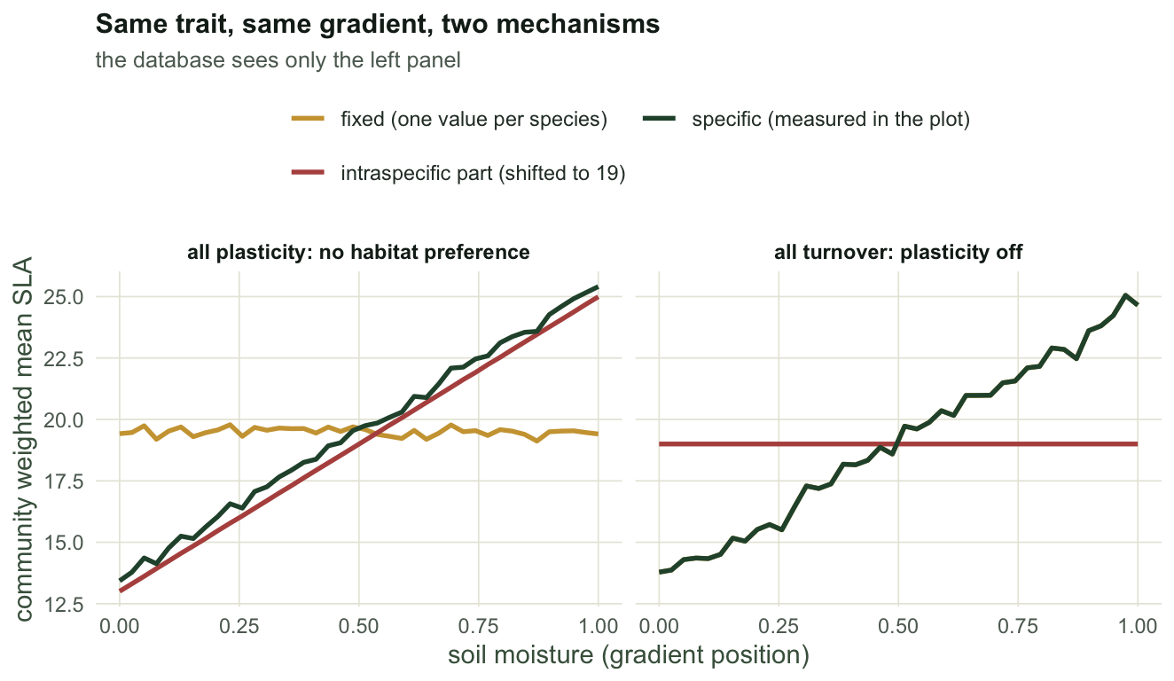
The mirror image is the one to worry about: a design where the species list does change, and the plants push back.
What the percentage table does when the two effects cancel
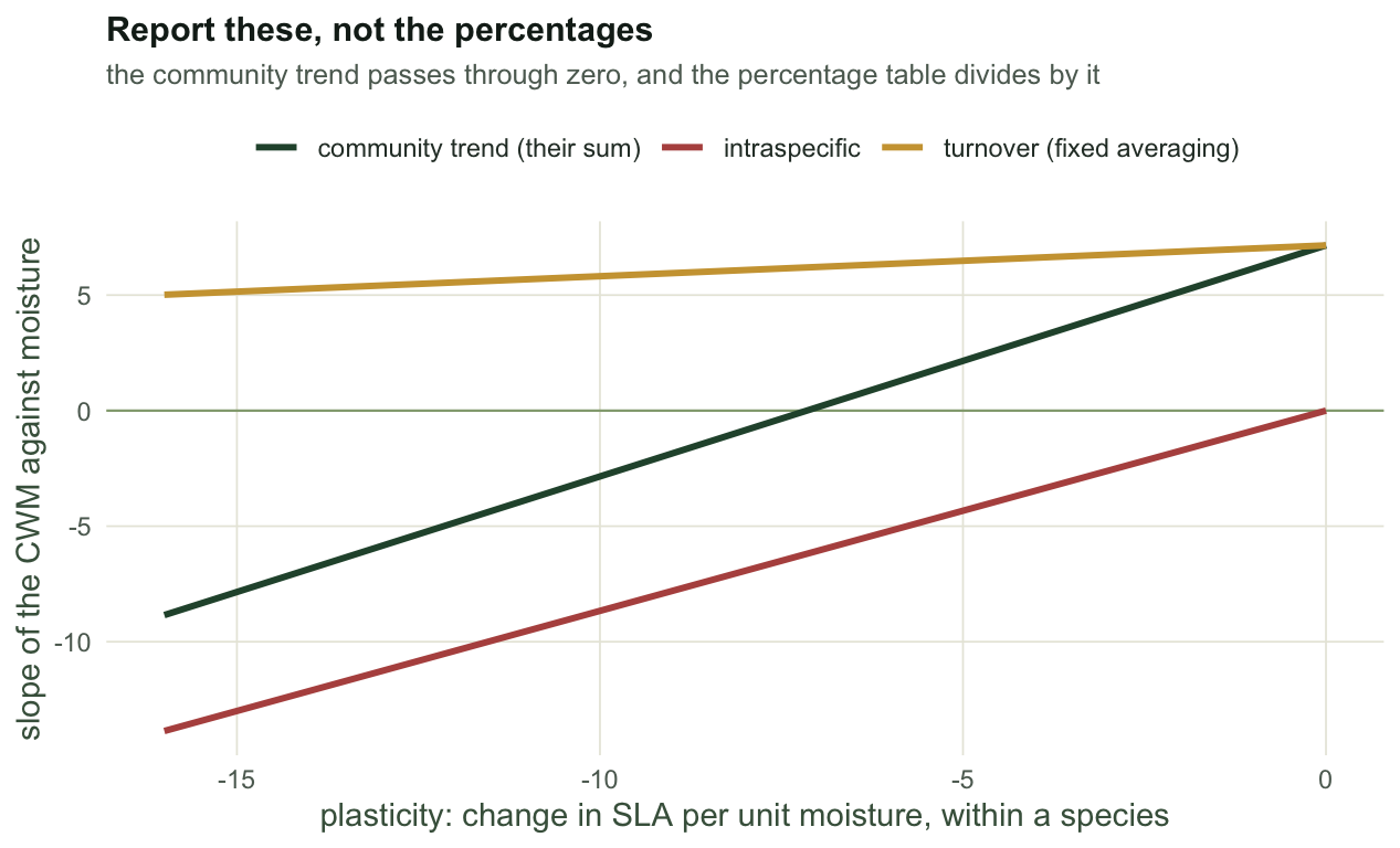
Give the species a moderate niche width, keep the turnover, and sweep the plasticity from zero to strongly compensating. The published output of the method is a percentage table, so build one:
gr <- c(0, -4, -8, -11, -14)
tab <- t(vapply(gr, function(pl) {
  s <- build(3091, tolr = 0.45, plast = pl); d <- unname(decomp(parts(s), s$e))
  ## decomp() order: turnover, intraspecific, covariation, total, b_fix, b_itv, b_spec, cross
  c(plasticity = pl, b_fix = d[5], b_itv = d[6], b_spec = d[7],
    pc_turnover = 100 * d[1] / d[4], pc_itv = 100 * d[2] / d[4], pc_cov = 100 * d[3] / d[4])
}, numeric(7)))
print(round(tab, 1))
plasticity b_fix b_itv b_spec pc_turnover pc_itv pc_cov
[1,] 0 7.2 0.0 7.2 100.0 0.0 0.0
[2,] -4 6.6 -3.5 3.2 440.9 120.9 -461.8
[3,] -8 6.1 -6.9 -0.8 5143.7 6678.1 -11721.8
[4,] -11 5.7 -9.5 -3.8 218.1 613.5 -731.6
[5,] -14 5.3 -12.1 -6.8 59.5 313.8 -273.3Read the table twice. The three slopes on the left move smoothly and stay additive: the fixed slope drifts a little, the intraspecific slope tracks the plasticity almost one for one, and their sum is the community trend. At a plasticity of -8 the table reports 5144% turnover, 6678% intraspecific and -11722% covariation, and they are not wrong: they sum to 100 exactly. They are ratios whose denominator is the variation the community trend explains, the square of its slope times the sum of squares of the gradient, and at that plasticity the slope is -0.85. A row that runs far outside nought to a hundred measures how nearly the two effects cancel, not how much each component contributed.
The split you report depends on niche breadth
The last measurement is the one that should change how the numbers are read. Hold the plasticity fixed at a single value, hold the base traits fixed, and vary only how wide a slice of the gradient each species occupies.
grid <- c(0.10, 0.14, 0.20, 0.28, 0.40, 0.55, 0.80, 1.20)
br <- t(vapply(grid, function(tl) {
  s <- build(3092, tolr = tl, plast = 8); p <- parts(s); d <- unname(decomp(p, s$e))
  cwo <- colSums(s$A * s$e) / colSums(s$A)                      # mean moisture per species
  brd <- mean(sqrt(colSums(s$A * (s$e - rep(cwo, each = nrow(s$A)))^2) / colSums(s$A)))
  c(tolerance = tl, niche_sd = brd, pc_turnover = 100 * d[1] / d[4], pc_itv = 100 * d[2] / d[4],
    intrinsic = bof(s$base, s$opt), from_survey = bof(p$spmn, s$opt))
}, numeric(6)))
print(round(br, 2))
tolerance niche_sd pc_turnover pc_itv intrinsic from_survey
[1,] 0.10 0.09 93.87 0.10 21.11 28.47
[2,] 0.14 0.12 87.51 0.42 21.11 28.04
[3,] 0.20 0.17 75.37 1.74 21.11 27.11
[4,] 0.28 0.21 58.73 5.46 21.11 25.93
[5,] 0.40 0.25 37.10 15.28 21.11 24.34
[6,] 0.55 0.27 21.26 29.04 21.11 23.20
[7,] 0.80 0.29 7.15 53.68 21.11 22.10
[8,] 1.20 0.29 1.90 74.34 21.11 21.54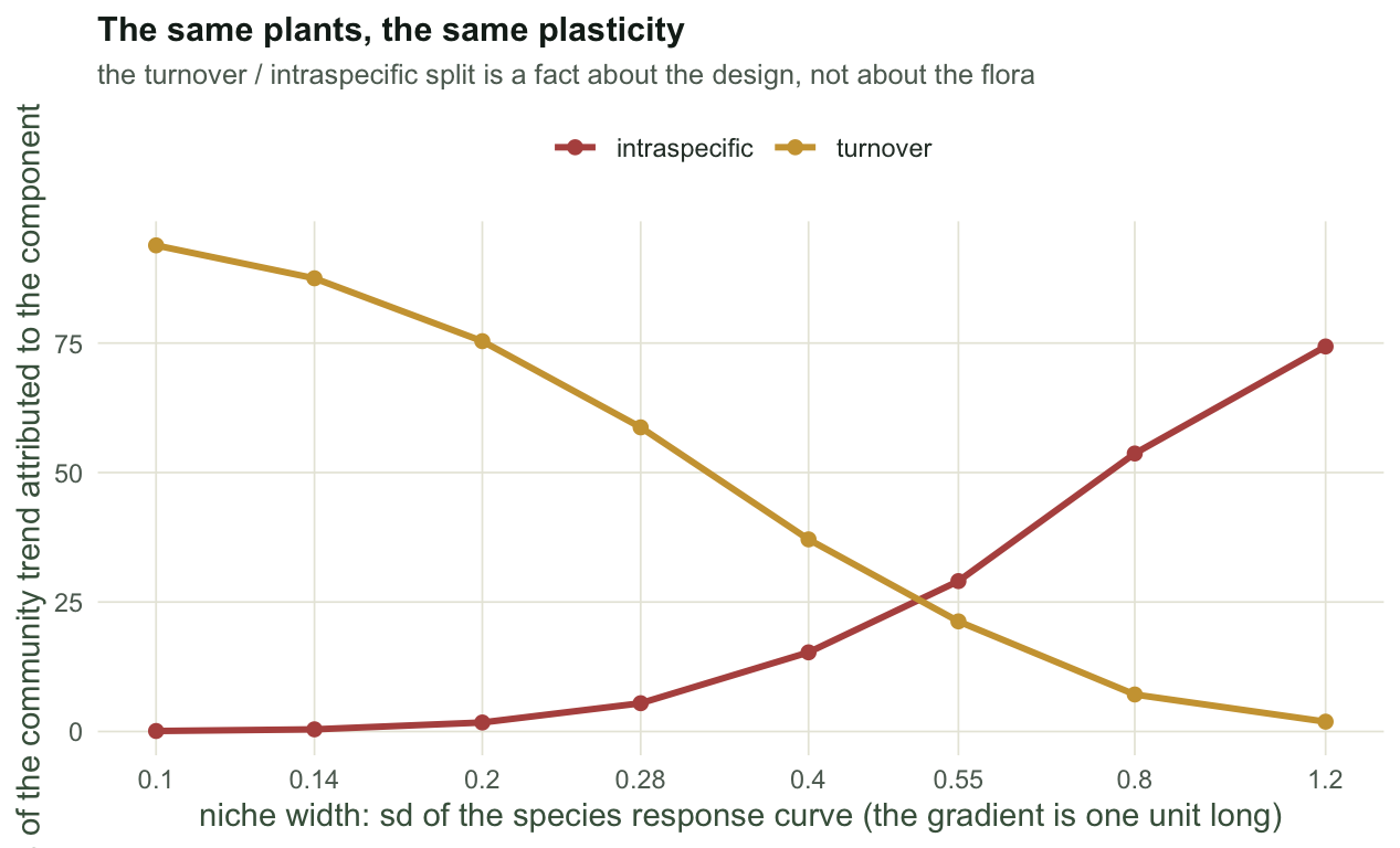
With narrow species the decomposition reports 94% turnover and 0.1% intraspecific. With wide species and the same plasticity it reports 2% and 74%. The mechanism is not subtle. A specialist is only ever measured near its own optimum, so its plot values sit close to its own mean, and there is nothing left over for the intraspecific term to hold. Plasticity that a species never expresses, because it never grows anywhere else, is invisible to a survey and correctly so.
The same sweep prices a second thing. The last two columns of the table regress the species trait against the species optimum, once on the intrinsic base values and once on the means the survey itself produces.
At the narrow end the intrinsic across species gradient is 21.1 and the survey returns 28.5. At the wide end the same two numbers are 21.1 and 21.5. A specialist’s trait value in a database is the value of a plant grown in the specialist’s own habitat, so part of what fixed averaging books as turnover is plasticity that was quietly absorbed into the species mean before the analysis started. No diagnostic in the decomposition can find it, because the intrinsic value was never measured.
What to report
- The three slopes, and their standard errors. They are additive, they are on the trait’s own scale, and they do not divide by anything.
- The percentages only when the community trend is clearly non zero, and with the trend printed next to them so a reader can see how near zero the denominator is.
- The niche breadth of your species along the gradient you are testing. In the sweep above it moved the split from almost all turnover to mostly intraspecific with plasticity held fixed, so two studies with different breadths are not comparable on the split alone.
- Whether the species means came from your own plots, from a regional database, or from a global one. Each choice moves a different amount of plasticity into the turnover column.
Where to go next
The decomposition needs the field measurements it is built to price. If you only have a database, the community weighted mean post is the honest limit of what you can compute, and the trait coverage arithmetic there applies before any of this does. If the question is whether the trait gradient exists at all rather than what drives it, the test comes with its own trouble, measured here. And the spread of trait values inside a plot, which both averagings discard, is functional diversity.
References
- Leps, de Bello, Smilauer & Dolezal 2011 Ecography 34(5):856-863 (10.1111/j.1600-0587.2010.06904.x)
- de Bello, Lavorel, Albert et al 2011 Methods in Ecology and Evolution 2(2):163-174 (10.1111/j.2041-210X.2010.00071.x)
- Albert, Grassein, Schurr, Vieilledent & Violle 2011 Perspectives in Plant Ecology, Evolution and Systematics 13(3):217-225 (10.1016/j.ppees.2011.04.003)
- Violle, Enquist, McGill et al 2012 Trends in Ecology & Evolution 27(4):244-252 (10.1016/j.tree.2011.11.014)
- Siefert, Violle, Chalmandrier et al 2015 Ecology Letters 18(12):1406-1419 (10.1111/ele.12508)