r4 <- function(E, T, L) {
  W <- sum(L); rs <- rowSums(L); cs <- colSums(L)
  Eb <- sum(rs * E) / W; Tb <- sum(cs * T) / W        # abundance-weighted means
  Ec <- E - Eb; Tc <- T - Tb
  cov <- as.numeric(Ec %*% L %*% Tc) / W               # weighted covariance
  vE  <- sum(rs * Ec^2) / W; vT <- sum(cs * Tc^2) / W  # weighted variances
  cov / sqrt(vE * vT)
}Fourth-corner trait-environment analysis
R
community ecology
functional ecology
traits
ecology tutorial
The fourth-corner statistic links species traits to the environment through abundance. Its naive permutation test over-rejects; the max-of-p fix controls it.
Corrected 7 October 2026: the introduction said the site-label permutation reports significance most of the time on any data without a trait-environment link; it now says this happens when species track the environment but the trait plays no part, as in the simulation below.
Functional ecology often asks a question with three tables in it. You have a site-by-species abundance table, a table of environmental conditions for the sites, and a table of traits for the species. The question is whether a trait modulates how species respond to the environment: do warm sites hold larger-bodied beetles, do wet sites hold species with a particular leaf habit. The fourth-corner statistic answers it by threading the trait table and the environment table through the abundance table, and it is one line of arithmetic once you see it as an abundance-weighted correlation.
The arithmetic is the easy part. The hard part is the test, and it is a genuine trap. The obvious permutation, shuffling site labels, can have a false-positive rate that is not a little too high but catastrophically too high: when species track the environment but the trait plays no part, it can report significance most of the time. This post builds the statistic by hand, shows the trap with a Monte Carlo study, and applies the fix from ter Braak, Cormont & Dray (2012).
The statistic
Write E for the environmental value at each site and T for the trait value of each species. The fourth-corner statistic is the correlation between E and T, computed across every site-by-species cell and weighted by the abundance in that cell. Cells with many individuals count more; empty cells count for nothing. In matrix form it is a weighted mean, a weighted covariance, and two weighted variances, all read off the abundance table.
The two permutations, and the trap
To get a p-value you need a null. Dray & Legendre (2008) set out the options as permutation models. Permuting site labels (their model 2) breaks the link between the environment and species composition. Permuting species labels (their model 4) breaks the link between traits and where species occur. The trouble is that a large statistic can arise for reasons that only one of these permutations controls: species may respond strongly to the environment for reasons unrelated to the trait, and a site-label permutation happily calls that significant even though it is not a trait-environment effect.
fourth_test <- function(E, T, L, B = 199, seed = 1) {
  set.seed(seed); obs <- abs(r4(E, T, L)); n <- nrow(L); S <- ncol(L)
  p2 <- (1 + sum(replicate(B, abs(r4(E, T, L[sample(n), , drop = FALSE]))) >= obs)) / (B + 1)
  p4 <- (1 + sum(replicate(B, abs(r4(E, T, L[, sample(S), drop = FALSE]))) >= obs)) / (B + 1)
  c(obs = obs, p2 = p2, p4 = p4, pmax = max(p2, p4))
}
The fix from ter Braak, Cormont & Dray (2012) is disarmingly simple: run both permutations and report the larger of the two p-values. A result is significant only when it survives shuffling sites and shuffling species, which is another way of saying the environment must be linked to composition and the trait must be linked to where species sit. That is exactly the joint claim a trait-environment effect makes.
Two datasets the naive test cannot be trusted to tell apart
Here are two simulated communities of 40 sites and 30 species. In both, species respond to the environment. In the first the trait is unrelated to that response, so there is no trait-environment effect. In the second the trait drives the response, so there is a real one.
gen <- function(seed, gamma = 0, n = 40, S = 30, size = 2) {
  set.seed(seed)
  E <- rnorm(n); T <- rnorm(S)
  cj   <- rnorm(S, log(c(rep(6,10), rep(2,10), rep(0.8,10))), 0.2)   # species abundances
  beta <- gamma * T + rnorm(S, 0, 0.9)                               # env-response of each species
  mu   <- exp(outer(rep(1,n), cj) + outer(E, beta))
  list(E = E, T = T, L = matrix(rnbinom(n*S, mu = as.vector(mu), size = size), n, S))
}
dn <- gen(seed = 11, gamma = 0)     # no trait-environment link
dr <- gen(seed = 11, gamma = 1.1)   # trait modulates the response
pn <- fourth_test(dn$E, dn$T, dn$L, B = 999, seed = 5)
pr <- fourth_test(dr$E, dr$T, dr$L, B = 999, seed = 5)
rbind(null = round(pn, 3), real = round(pr, 3))
obs p2 p4 pmax
null 0.287 0.001 0.255 0.255
real 0.663 0.001 0.001 0.001Look at the naive site-permutation column. It returns 0.001 for the null dataset and 0.001 for the real one. Whatever those two numbers come out at, the site-label permutation is only asking whether composition tracks the environment, which is true in both datasets by construction, so a small p-value from it is not evidence of a trait effect. On its own it cannot be relied on to separate a real trait-environment effect from a species-responds-to-environment artefact. The max-of-p column does the job it was asked to do: 0.255 for the null, not significant, and 0.001 for the real effect. The difference comes entirely from the species permutation, which finds no trait link in the first dataset and a clear one in the second.
How often the naive test cries wolf
One pair of datasets could be luck. A Monte Carlo study settles it: 300 null communities, no trait-environment link in any of them, each tested three ways.
M <- 300; n <- 40; S <- 30; B <- 199
p2v <- p4v <- pmv <- numeric(M)
for (m in 1:M) {
  d <- gen(seed = 1000 + m, gamma = 0, n = n, S = S)
  pv <- fourth_test(d$E, d$T, d$L, B = B, seed = m)
  p2v[m] <- pv["p2"]; p4v[m] <- pv["p4"]; pmv[m] <- pv["pmax"]
}
rate2 <- mean(p2v < 0.05); rate4 <- mean(p4v < 0.05); ratem <- mean(pmv < 0.05)
c(sites_only = round(rate2, 3), species_only = round(rate4, 3), max_of_p = round(ratem, 3))
sites_only species_only max_of_p
0.72 0.05 0.05 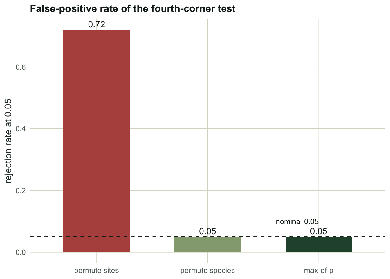
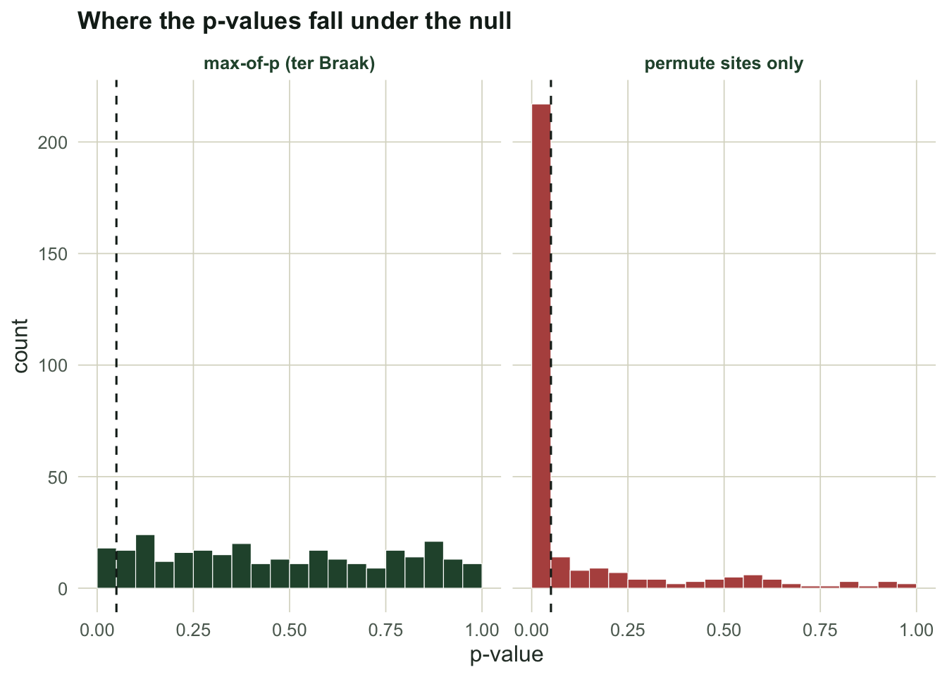
Permuting sites rejects a true null 72 per cent of the time. Permuting species, and the max-of-p that inherits its calibration, both sit on the nominal 0.05. The p-value histogram shows the mechanism directly: a valid test spreads its p-values evenly between zero and one, while the site-only test dumps them against zero.
Honest limits
The max-of-p fix buys valid Type-I error at a price in power, since a real effect now has to clear two hurdles rather than one; that is the right trade, but it is a trade. The statistic itself is a correlation, so it sees linear trait-environment relationships and will miss a hump-shaped one unless you build the shape in. A significant fourth corner is an association, not a mechanism: the trait may be standing in for phylogeny or for another trait it happens to correlate with, and only a design that varies the trait can promote the pattern to a cause, the same caution as the observational tools elsewhere on this site. With several traits and several environmental variables the cells multiply, and the family of tests needs false-discovery control before you read the stars. Within those limits the message is clean and worth carrying: the intuitive permutation is the wrong one, it fails loudly rather than quietly, and reporting the larger of two p-values is what makes the test mean what it claims.
References
Legendre P, Galzin R, Harmelin-Vivien ML 1997. Ecology 78:547-562 (10.1890/0012-9658(1997)078[0547:RBTHST]2.0.CO;2).
Doledec S, Chessel D, ter Braak CJF, Champely S 1996. Environmental and Ecological Statistics 3:143-166 (10.1007/BF02427859).
Dray S, Legendre P 2008. Ecology 89:3400-3412 (10.1890/08-0349.1).
ter Braak CJF, Cormont A, Dray S 2012. Ecology 93:1525-1526 (10.1890/12-0126.1).
Brown AM, Warton DI, Andrew NR, Binns M, Cassis G, Gibb H 2014. Methods in Ecology and Evolution 5:344-352 (10.1111/2041-210X.12163).