Model-based multivariate abundance

Distance-based community methods confound the mean-variance relationship with real composition change. Model each species with a GLM, and test the community by resampling.

Ordination and PERMANOVA on a Bray-Curtis matrix are the reflexive first move for community data. Both start by turning a site-by-species table into pairwise dissimilarities, and that step quietly makes a strong assumption: how much a species contributes to the distance depends on its variance, and for count data the variance is tied to the mean. A rare species and a common one carry different weight for reasons that have nothing to do with ecology.

The model-based alternative keeps every species on its own scale. Fit one generalised linear model per species with a shared set of predictors, then test the community by resampling. That single change separates two things a dissimilarity matrix mixes together: a shift in the mean (which species are more or less abundant) and a shift in dispersion (how variable the assemblage is). This post builds the community test by hand and shows the confounding that motivates it.

A community with a real change in the mean

We simulate 25 sites in each of two groups, Control and Impact, and 20 species along an abundant-to-rare gradient. The impact is an abundance reduction: most species fall to 30 per cent of their control mean, and four sensitive species fall further, so the composition changes as well. Crucially the negative binomial size parameter is the same in both groups, so there is no genuine change in dispersion built into the data. Any dispersion signal we later detect on Bray-Curtis is therefore an artefact.

set.seed(4222)
S     <- 20
n_per <- 25
grp   <- factor(rep(c("Control", "Impact"), each = n_per),
                levels = c("Control", "Impact"))
n     <- length(grp)

base_mu   <- c(rep(14, 3), rep(7, 5), rep(3, 7), rep(1.1, 5))  # control means
mult      <- rep(0.30, S)                                      # impact: abundance reduction
mult[1:4] <- 0.12                                              # four sensitive species
theta_true <- 2                                               # NB size, identical in both groups

mu_mat <- outer(rep(1, n), base_mu)
mu_mat[grp == "Impact", ] <- sweep(mu_mat[grp == "Impact", ], 2, mult, "*")
Y <- matrix(rnbinom(n * S, mu = as.vector(mu_mat), size = theta_true), n, S)
colnames(Y) <- paste0("sp", 1:S)

mean_ctrl  <- mean(Y[grp == "Control", ])
mean_imp   <- mean(Y[grp == "Impact", ])
ratio_mean <- mean_imp / mean_ctrl
zeros_ctrl <- 100 * mean(Y[grp == "Control", ] == 0)
zeros_imp  <- 100 * mean(Y[grp == "Impact", ] == 0)
c(mean_ctrl = mean_ctrl, mean_imp = mean_imp, ratio = ratio_mean)

mean_ctrl  mean_imp     ratio 
5.5360000 1.0880000 0.1965318 

The impact sites average 1.09 individuals per species against 5.54 in the controls, a ratio of 0.2, and they carry many more zeros (45 per cent against 16 per cent).

The mean-variance relationship is the whole problem

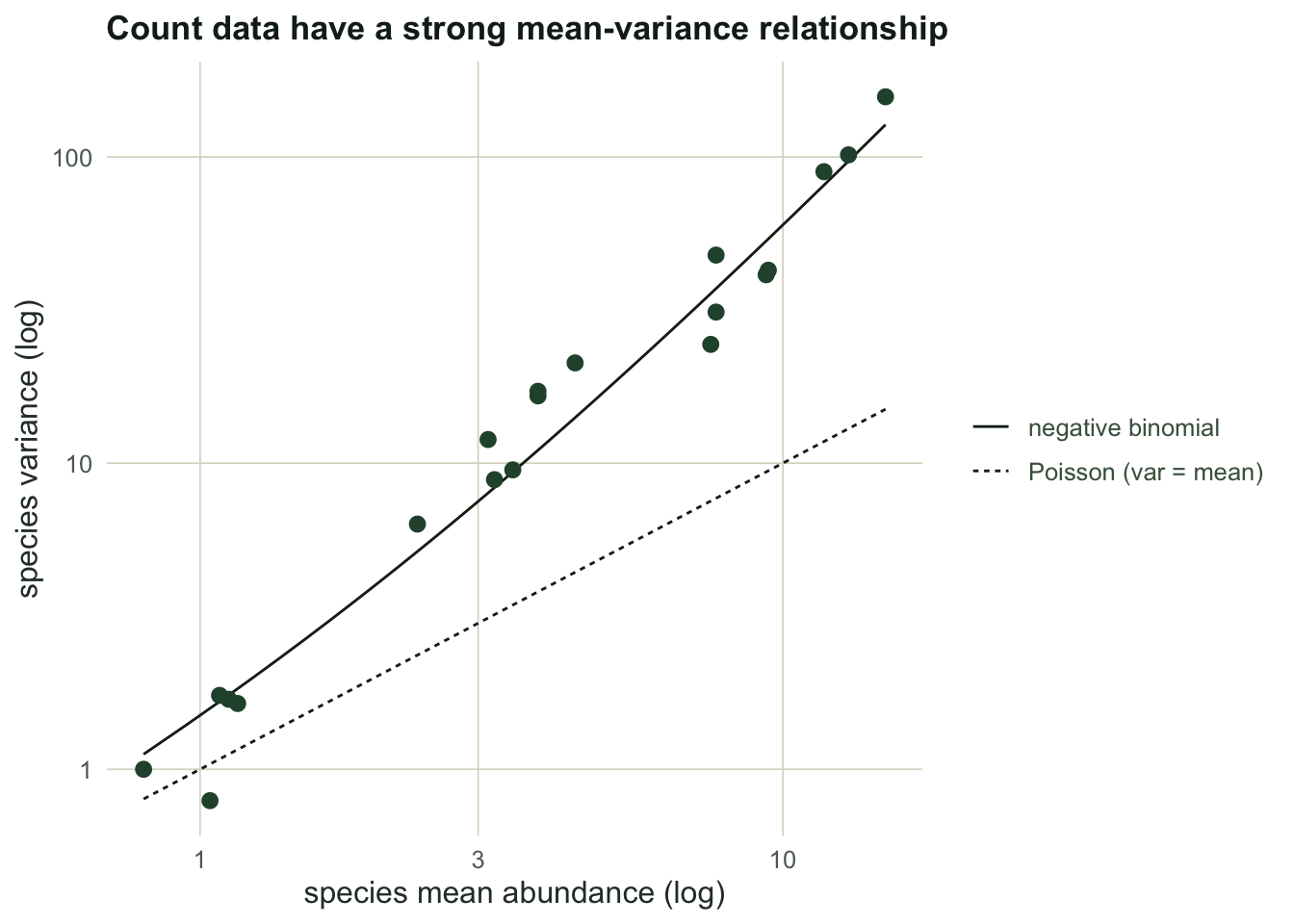
For each species, take its mean and its variance across the control sites and plot one against the other on log axes. Count data sit near a line steeper than the Poisson one-to-one reference: the variance grows roughly with the square of the mean, the signature of overdispersion.

sp_mean  <- colMeans(Y[grp == "Control", ])
sp_var   <- apply(Y[grp == "Control", ], 2, var)
mv_slope <- coef(lm(log(sp_var) ~ log(sp_mean)))[2]
round(mv_slope, 3)

log(sp_mean) 
        1.67 

Figure 1: Each point is a species. Distance measures ignore this relationship; a GLM writes it into the likelihood.

The log-log slope here is 1.67, between the Poisson value of one and the quadratic value of two. Bray-Curtis has no way to know this. It treats a difference of ten individuals in a common species and in a rare one on comparable footing, so the abundant species dominate the dissimilarities, and the relationship in the figure leaks into the analysis as if it were signal.

The community test, by hand

A model-based analysis fits a separate negative binomial GLM to each species, y ~ group, and compares it to the null y ~ 1. The likelihood-ratio statistic for each species measures how much the group improves the fit, and the community statistic is their sum. We first estimate each species’ dispersion once from the full data, then hold it fixed, so the test is a clean comparison of the group term and the permutations below are fast.

theta_hat <- numeric(S)
for (s in 1:S) {
  fit <- tryCatch(glm.nb(Y[, s] ~ grp), error = function(e) NULL)
  theta_hat[s] <- if (is.null(fit)) 1e6 else fit$theta
}

lr_species <- function(y, g, th) {
  f1 <- glm(y ~ g, family = negative.binomial(th))
  f0 <- glm(y ~ 1, family = negative.binomial(th))
  as.numeric(deviance(f0) - deviance(f1))
}
LR_obs    <- sapply(1:S, function(s) lr_species(Y[, s], grp, theta_hat[s]))
Tcomm_obs <- sum(LR_obs)
round(Tcomm_obs, 1)

[1] 611.2

The null distribution needs the right exchangeable unit. Species are correlated, so shuffling them one at a time would destroy the between-species structure and give the wrong error rate. Instead we permute the group labels, which keeps every site’s full species vector intact and only breaks the link between sites and groups. Under the null of no group effect the labels are exchangeable, and each permutation gives one draw from the community statistic under that null.

B <- 999
Tperm <- numeric(B)
for (b in 1:B) {
  gp <- sample(grp)
  Tperm[b] <- sum(sapply(1:S, function(s) lr_species(Y[, s], gp, theta_hat[s])))
}
p_comm <- (1 + sum(Tperm >= Tcomm_obs)) / (B + 1)
c(observed = round(Tcomm_obs, 1), max_null = round(max(Tperm), 1), p = p_comm)

observed max_null        p 
 611.200  156.600    0.001 

The observed community statistic is 611, the largest of 999 permuted values is 157, and the resampled p-value is below 0.001. The group effect is real, which we know because we built it in. Holding the dispersion fixed at each species’ own estimate lets a common species and a rare one both speak, weighted by how much information each actually carries.

The confound: a mean shift fakes a dispersion difference

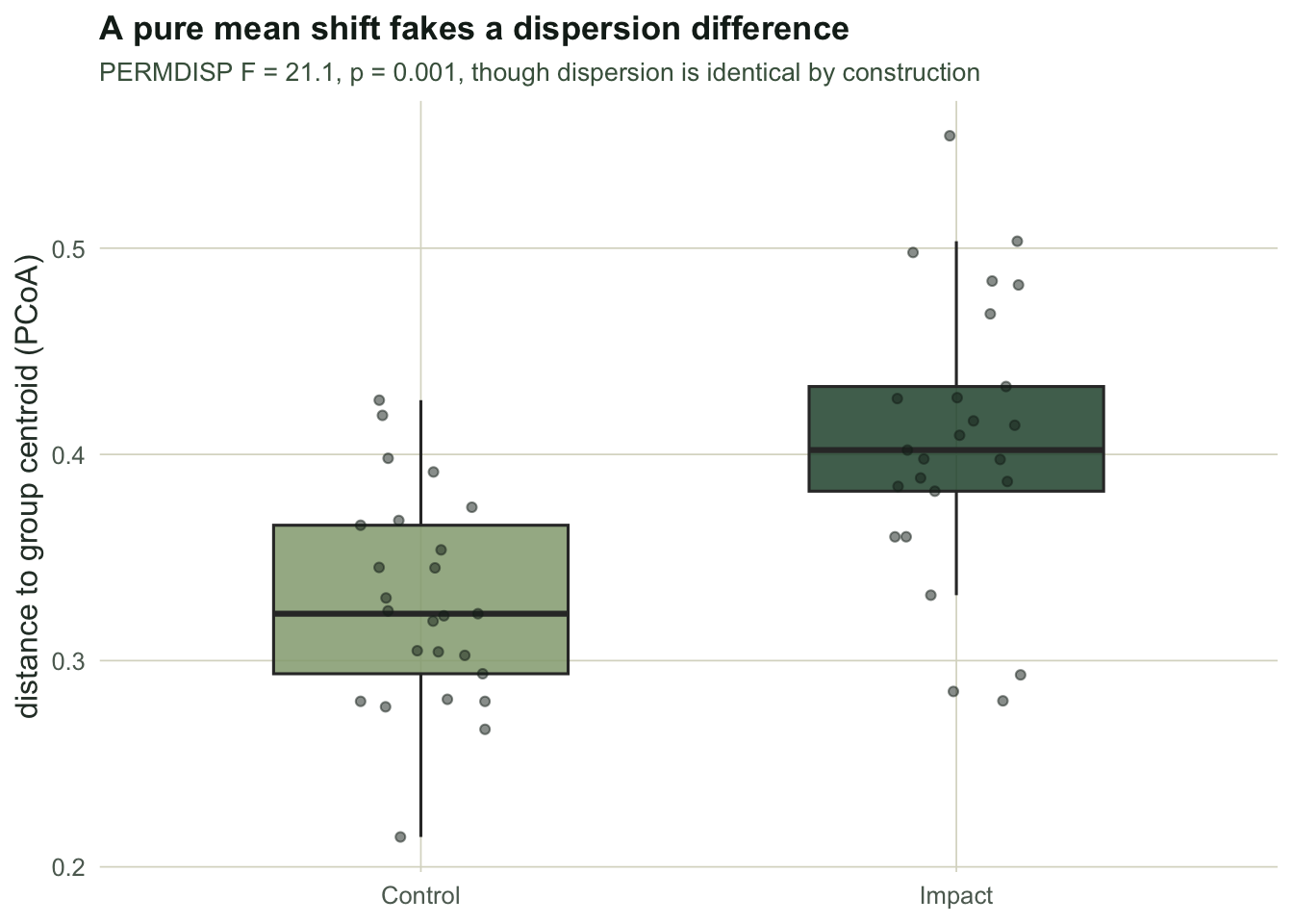
Now run the distance-based analysis and check what it reports. We build the Bray-Curtis matrix by hand, place the sites in Euclidean space with principal coordinates, and measure each site’s distance to its group centroid. That distance is the multivariate dispersion, and the permutation test on it is the distance-based analogue of a variance test.

bray <- function(M) {
  n <- nrow(M); D <- matrix(0, n, n)
  for (i in 1:(n - 1)) for (j in (i + 1):n) {
    d <- sum(abs(M[i, ] - M[j, ])) / sum(M[i, ] + M[j, ]); D[i, j] <- D[j, i] <- d
  }
  D
}
D  <- bray(Y)
G  <- { A <- -0.5 * D^2; Cn <- diag(n) - matrix(1/n, n, n); Cn %*% A %*% Cn }
ev <- eigen(G, symmetric = TRUE)
X  <- ev$vectors[, ev$values > 1e-8] %*% diag(sqrt(ev$values[ev$values > 1e-8]))

dcen <- numeric(n)
for (lev in levels(grp)) {
  idx <- grp == lev; ctr <- colMeans(X[idx, , drop = FALSE])
  dcen[idx] <- sqrt(rowSums(sweep(X[idx, , drop = FALSE], 2, ctr)^2))
}
permdisp_F <- function(d, g) {
  gm <- tapply(d, g, mean); grand <- mean(d)
  ssb <- sum(table(g) * (gm - grand)^2); ssw <- sum((d - gm[as.character(g)])^2)
  (ssb / (nlevels(g) - 1)) / (ssw / (length(d) - nlevels(g)))
}
F_obs  <- permdisp_F(dcen, grp)
Fp     <- replicate(999, permdisp_F(dcen, sample(grp)))
p_disp <- (1 + sum(Fp >= F_obs)) / 1000
disp_ctrl <- mean(dcen[grp == "Control"]); disp_imp <- mean(dcen[grp == "Impact"])
c(disp_ctrl = round(disp_ctrl, 3), disp_imp = round(disp_imp, 3),
  F = round(F_obs, 1), p = p_disp)

disp_ctrl  disp_imp         F         p 
    0.328     0.407    21.100     0.001 

Figure 2: Only the mean changed in the data, yet the distance-based test reads it as a dispersion difference.

The impact sites sit at mean distance 0.407 from their centroid against 0.328 for the controls, and the dispersion test returns F = 21.1 with p = 0.001. Read at face value this says the impacted community is more heterogeneous, perhaps destabilised. It is nothing of the sort. The dispersion parameter is identical in both groups; the only thing that changed is the mean. Lower counts carry proportionally more sampling variability and more zeros, so Bray-Curtis distances stretch, and the variance test picks that up as dispersion. The model-based analysis attributes the same data to the mean, where it belongs, and its p-value of 0.001 reflects a location effect, not a dispersion one.

This is the same trap as testing dispersion after PERMANOVA: a significant PERMDISP result can be a mean effect wearing a dispersion costume, and the reverse is possible too.

Honest limits

The community test tells you the assemblage responds to the grouping. It does not tell you which species drive it; the per-species statistics need multiple-testing control before you read them, which is the subject of a later post. It also assumes the mean-variance relationship you fit, and if the negative binomial is wrong the test is not valid, so the residual check matters. And the framing is not settled: Roberts (2017) argued that distance measures are not simply wrong, and that their implied mean-variance ratio can be defensible, so the choice between the two families is partly about what question you are asking. What is not in dispute is that a Bray-Curtis dispersion result should never be read as an ecological dispersion effect without ruling out a mean shift first.

References

Warton DI, Wright ST, Wang Y 2012. Distance-based multivariate analyses confound location and dispersion effects. Methods in Ecology and Evolution 3:89-101 (10.1111/j.2041-210X.2011.00127.x).

Wang Y, Naumann U, Wright ST, Warton DI 2012. mvabund: an R package for model-based analysis of multivariate abundance data. Methods in Ecology and Evolution 3:471-474 (10.1111/j.2041-210X.2012.00190.x).

Roberts DW 2017. Distance, dissimilarity, and mean-variance ratios in ordination. Methods in Ecology and Evolution 8:1508-1514 (10.1111/2041-210X.12739).

Anderson MJ 2001. A new method for non-parametric multivariate analysis of variance. Austral Ecology 26:32-46.

McArdle BH, Anderson MJ 2001. Fitting multivariate models to community data: a comment on distance-based redundancy analysis. Ecology 82:290-297.

Taylor LR 1961. Aggregation, variance and the mean. Nature 189:732-735 (10.1038/189732a0).

Related tutorials

• Common PERMANOVA mistakes
• Model-based unconstrained ordination
• Fourth-corner trait-environment analysis
• Checking a model-based multivariate model