library(vegan)
library(ggplot2)

## mean-corrected lognormal abundances: E[abundance] = lambda for every group,
## so groups can share an identical expected composition while differing only in spread
gen_group <- function(n, sig, lambda) {
  nsp <- length(lambda)
  M <- matrix(0, n, nsp)
  for (i in 1:n) M[i, ] <- round(lambda * exp(rnorm(nsp, 0, sig) - sig^2 / 2))
  M[M < 0] <- 0
  M
}Four common PERMANOVA mistakes in ecology
R
vegan
multivariate
PERMANOVA
ecology tutorial
A significant PERMANOVA can really be unequal dispersion. Check betadisper, pick the right dissimilarity, respect your design, and read adonis2 honestly.
Step 20 of the Tidy Ecology course, Part four: find the structure.
Updated 27 September 2026: Mistake 4 now says to run the dispersion test with bias.adjust = TRUE when group sizes are unequal, and that even then a non-significant dispersion test can miss a small group that is modestly more dispersed, as a new post on betadisper with unequal group sizes measures; the rule under Mistake 1 now says it holds for balanced groups; and a new section, Before any of them: empty samples, measures what the usual repairs for an empty sample do to the test.
Corrected 25 September 2026: Mistake 3 said free permutation in a repeated-measures design is usually anticonservative. Which way it errs depends on the term: it flatters a treatment applied to whole sites and is too strict for a term that varies within sites. The passage now says so and points to a post that measures both.
PERMANOVA, run through vegan::adonis2, is the default tool for asking whether community composition differs between groups. It is powerful, assumption-light, and easy to call, which is exactly why it is so often misread. A small p value feels like a clean verdict that composition differs. It is not, on its own, any such thing. This post works through the four mistakes that most often turn a PERMANOVA into a confident wrong conclusion, with the first one being by far the most important.
Mistake 1: reading a significant result as a location difference
PERMANOVA partitions the total sum of squared dissimilarities into a between-group and a within-group part and forms a pseudo-F. The trouble is that the between-group term responds to two quite different things at once: a shift in the group centroids (a location, or composition, difference, which is what you usually mean), and a difference in how spread out the groups are (a dispersion, or beta-diversity, difference). A pseudo-F can be large because the centroids moved, because one group is far more variable than the other, or both. The test alone cannot tell you which.
This matters because the two have completely different ecological meanings, and because of a subtle geometric fact: in Bray-Curtis space, groups with identical mean abundances but different dispersions develop genuinely separated centroids. Anderson and Walsh demonstrate this directly; unequal variability in the original abundance space shows up partly as a centroid shift once you compute dissimilarities. So a dispersion difference does not just inflate the residual; it leaks into the between-group term and can make PERMANOVA reject when nothing about the mean composition changed.
Here are two groups drawn from the same twelve-species mean-abundance vector. The only difference is that group B is far more variable from site to site.
set.seed(101)
nsp <- 12
lambda1 <- exp(seq(log(3), log(45), length.out = nsp))
Y1 <- rbind(gen_group(30, 0.30, lambda1),   # group A: tight
            gen_group(30, 1.10, lambda1))   # group B: diffuse, identical expected composition
g1 <- factor(rep(c("A", "B"), each = 30))
D1 <- vegdist(Y1, method = "bray")
Run PERMANOVA, then immediately run the dispersion test that should always accompany it, betadisper.
ad1 <- adonis2(D1 ~ g1, permutations = 999)
c(F = round(ad1$F[1], 2), R2 = round(ad1$R2[1], 3), p = ad1$`Pr(>F)`[1])
F R2 p
4.640 0.074 0.001 bd1 <- betadisper(D1, g1)
an1 <- anova(bd1)
c(F = round(an1$`F value`[1], 1), p = signif(an1$`Pr(>F)`[1], 3)) F p
2.108e+02 5.720e-21 round(tapply(bd1$distances, g1, mean), 3) # mean distance to group centroid A B
0.110 0.349 PERMANOVA returns a significant result (p around 0.001) with an R squared of about 0.07. Taken alone you would report that composition differs between groups. But betadisper is overwhelmingly significant, with an F over 200, and the mean distance to centroid is 0.11 for group A against 0.35 for group B. The groups are not centred in different places by design; one is simply three times more dispersed than the other, and that heterogeneity is what PERMANOVA picked up. The small R squared is the tell: a real composition shift of ecological interest rarely hides at 7 per cent while the dispersion test screams.
Now the honest case: a real composition shift, with dispersion held equal.
set.seed(202)
lambdaA <- exp(seq(log(3), log(45), length.out = nsp))
lambdaB <- lambdaA
lambdaB[1:4] <- lambdaB[1:4] * 4     # boost the rare species
lambdaB[9:12] <- lambdaB[9:12] / 4   # suppress the common ones
Y2 <- rbind(gen_group(30, 0.6, lambdaA),
            gen_group(30, 0.6, lambdaB))   # same sigma in both groups
g2 <- factor(rep(c("A", "B"), each = 30))
D2 <- vegdist(Y2, method = "bray")
ad2 <- adonis2(D2 ~ g2, permutations = 999)
c(F = round(ad2$F[1], 2), R2 = round(ad2$R2[1], 3), p = ad2$`Pr(>F)`[1]) F R2 p
49.070 0.458 0.001 bd2 <- betadisper(D2, g2)
an2 <- anova(bd2)
c(F = round(an2$`F value`[1], 2), p = round(an2$`Pr(>F)`[1], 2)) F p
0.38 0.54 round(tapply(bd2$distances, g2, mean), 3) A B
0.243 0.234 This is what a trustworthy result looks like. PERMANOVA is strongly significant with an R squared of 0.46, and betadisper is non-significant (p around 0.54) with near-identical spreads (0.24 and 0.23). The centroids genuinely moved and the clouds are equally tight, so the PERMANOVA result means what you want it to mean.
The picture makes the contrast immediate.
pco <- function(D, g, lab) {
  cs <- cmdscale(D, k = 2)
  data.frame(ax1 = cs[, 1], ax2 = cs[, 2], grp = g, panel = lab)
}
od <- rbind(pco(D1, g1, "dispersion artefact"),
            pco(D2, g2, "true location shift"))
od$panel <- factor(od$panel, levels = c("dispersion artefact",
                                         "true location shift"))
cent <- aggregate(cbind(ax1, ax2) ~ grp + panel, od, mean)
ggplot(od, aes(ax1, ax2, colour = grp)) +
  geom_point(alpha = 0.6, size = 1.8) +
  geom_point(data = cent, size = 5, shape = 17) +
  facet_wrap(~panel, scales = "free") +
  scale_colour_manual(values = c(A = "#275139", B = "#cda23f"), name = "group") +
  labs(x = "PCoA 1", y = "PCoA 2") +
  theme_minimal(base_size = 12) +
  theme(panel.grid.minor = element_blank(),
        strip.text = element_text(colour = "#16241d", face = "bold"),
        plot.background = element_rect(fill = "#f5f4ee", colour = NA),
        panel.background = element_rect(fill = "#f5f4ee", colour = NA))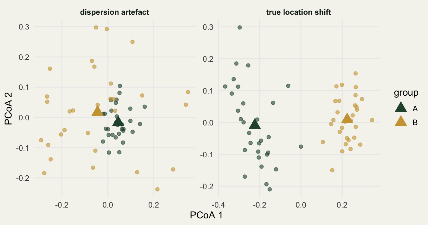
The triangles are the group centroids. On the left they sit almost on top of each other, yet the gold cloud sprawls while the green one is compact: that asymmetry is the whole of the PERMANOVA signal. On the right the centroids are pulled clearly apart and the two clouds are equally tight. The betadisper distances draw the same conclusion as a one-dimensional summary.
dd <- rbind(
  data.frame(dist = bd1$distances, grp = g1, panel = "dispersion artefact"),
  data.frame(dist = bd2$distances, grp = g2, panel = "true location shift"))
dd$panel <- factor(dd$panel, levels = c("dispersion artefact",
                                        "true location shift"))
ggplot(dd, aes(grp, dist, fill = grp)) +
  geom_boxplot(width = 0.55, colour = "#16241d", outlier.size = 0.8) +
  facet_wrap(~panel) +
  scale_fill_manual(values = c(A = "#275139", B = "#cda23f"), guide = "none") +
  labs(x = NULL, y = "distance to centroid") +
  theme_minimal(base_size = 12) +
  theme(panel.grid.minor = element_blank(),
        strip.text = element_text(colour = "#16241d", face = "bold"),
        plot.background = element_rect(fill = "#f5f4ee", colour = NA),
        panel.background = element_rect(fill = "#f5f4ee", colour = NA))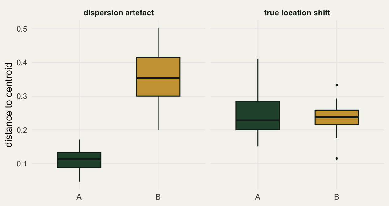
The rule is simple: never report a PERMANOVA without the matching betadisper. A significant PERMANOVA with a significant dispersion test is ambiguous, and you must say so. A significant PERMANOVA with a non-significant dispersion test is a clean location difference (with balanced groups; see Mistake 4 for unequal ones).
Mistake 2: the wrong dissimilarity
PERMANOVA works on whatever dissimilarity matrix you hand it, and the choice is not a formality. Euclidean distance on raw abundances, the implicit default if you reach for dist, is almost always wrong for community data. It treats two joint absences as evidence of similarity (the double-zero problem), it is dominated by the most abundant species, and it has no upper bound, so a single superabundant taxon can swamp everything else.
D_bray <- vegdist(Y2, method = "bray")   # appropriate for composition
D_euc  <- dist(Y2)                        # raw Euclidean, the wrong default
c(bray_R2 = round(adonis2(D_bray ~ g2, permutations = 999)$R2[1], 3),
  euclidean_R2 = round(adonis2(D_euc ~ g2, permutations = 999)$R2[1], 3))
bray_R2 euclidean_R2
0.458 0.359 On the very same data the two measures attribute different amounts of variation to the grouping (0.46 against 0.36 here), and on more skewed data they routinely disagree about significance itself. Use Bray-Curtis or Jaccard for abundances, Jaccard or Sorensen for presence-absence, or a Hellinger transformation followed by Euclidean distance if you want a transformation-based RDA-compatible metric. Match the dissimilarity to the data; do not let dist decide for you.
Mistake 3: ignoring the design when permuting
PERMANOVA gets its p value by shuffling labels. The default shuffles freely, which is only valid if every sampling unit is exchangeable under the null. The moment your design has structure, repeated measures on the same plots, subplots nested in sites, a blocked or split-plot layout, free permutation tests the wrong hypothesis, and which way it errs depends on the term: a term that is constant within a site, such as a site-level treatment, gets significance it did not earn and has to be tested by shuffling whole sites, while a term that varies within sites, such as year in a repeated survey, is held to so strict a standard that a real effect can go undetected. The blocked call below is for the second kind (on a site-level treatment it cannot move a single label and returns the largest possible p value), as the post on repeated-measures PERMANOVA measures.
The fix is to restrict the permutations to the exchangeable structure using how from the permute package, which adonis2 accepts directly.
library(permute)
# treatment applied to subplots nested in 'site'; permute only within sites
ctrl <- how(blocks = site, nperm = 999)
adonis2(D ~ treatment, permutations = ctrl)
Restricting the permutations leaves the observed pseudo-F unchanged but builds the null distribution from rearrangements the design actually permits, which is the only valid reference. If you have repeated measures or nesting and you are permuting freely, your p value is answering a question you did not ask.
Mistake 4: unbalanced groups plus unequal dispersion
The dispersion problem of mistake 1 gets sharper when group sizes are unequal. Anderson and Walsh’s simulations show that with unbalanced designs the tests are too liberal when the smaller group is the more dispersed one, and too conservative when the larger group is. In other words, a small, noisy group can manufacture a significant PERMANOVA out of pure dispersion, and you will not see it unless you have checked balance and run betadisper. Aim for balanced designs where you can; where you cannot, treat a significant result with heterogeneous dispersions and unequal n with real suspicion, and lean on the dispersion test to interpret it, run with bias.adjust = TRUE: with the default, betadisper underestimates the dispersion of a small group, so it flags differences that are not there and is least sensitive when the small group is somewhat more dispersed. Even adjusted, read a non-significant dispersion test with care: it can still miss a small group that is modestly more dispersed, and so let through many of the false PERMANOVA results it was meant to catch (betadisper with unequal group sizes).
Before any of them: empty samples
The four mistakes assume that every sample holds at least one individual. Field data often do not: a pitfall trap that caught nothing, a quadrat on bare rock, a grab from a denuded patch. Bray-Curtis standardises by the two sample totals (the property that choosing a dissimilarity index describes), so an empty sample is a problem for the dissimilarity before it is one for PERMANOVA. Four samples from each group of the location-shift data, plus one and then two empty samples, show what vegdist() does.
warned <- function(expr) { msgs <- character(0)   # keep the value, collect the warnings
  value <- withCallingHandlers(expr, warning = function(w) { msgs <<- c(msgs, gsub("\\s+", " ", conditionMessage(w)))
    invokeRestart("muffleWarning") }); list(value = value, warnings = msgs) }
Y_two <- rbind(Y2[c(1:4, 31:34), ], 0, 0)   # four samples per group, then two empty ones
g_two <- factor(c(as.character(g2[c(1:4, 31:34)]), "B", "B"))
bc_one <- warned(vegdist(Y_two[1:9, ], method = "bray"))
bc_two <- warned(vegdist(Y_two, method = "bray"))
stopifnot(all(as.matrix(bc_one$value)[9, -9] == 1), is.nan(as.matrix(bc_two$value)[9, 10]),
          any(grepl("empty rows", bc_one$warnings)), any(grepl("missing values in results", bc_two$warnings)))
bc_two$warnings
[1] "you have empty rows: their dissimilarities may be meaningless in method \"bray\""
[2] "missing values in results" set.seed(303)
ad_two <- tryCatch(adonis2(bc_two$value ~ g_two, permutations = 199), error = function(e) e)
adonis_failed <- inherits(ad_two, "error")
c(vegan = packageDescription("vegan")$Version, adonis2 = if (adonis_failed) conditionMessage(ad_two) else "ran") vegan adonis2
"2.7-5" "missing value where TRUE/FALSE needed" M_dummy <- as.matrix(vegdist(cbind(Y_two, 1), method = "bray")) # dummy species of 1
tot <- rowSums(Y_two)[1:8]
stopifnot(M_dummy[9, 10] == 0,
isTRUE(all.equal(M_dummy[9, 1:8], tot / (tot + 2), check.attributes = FALSE)))With one empty sample, its dissimilarity to every other sample is exactly 1, and vegdist() warns that the dissimilarities of empty rows “may be meaningless”. With two, the dissimilarity between the two empty samples is 0 divided by 0, stored as NaN, and a second warning follows. adonis2() then stops with the error printed above, which says nothing about empty samples (vegan 2.7-5 here; other versions may word it differently). Three repairs are common: drop the empty samples; set the NaN to 0, which declares two empty samples identical; or use the zero-adjusted Bray-Curtis of Clarke et al. (2006), which adds a dummy species to every sample; here it is a count of 1, the smallest non-zero count (cbind(Y, 1)). The dummy also makes two empty samples identical, and it puts an empty sample at T/(T + 2) from a sample of T individuals: 0.981 to 0.993 for the well-stocked samples above, but a third for a sample of one individual. It leaves rich samples almost alone and pulls sparse ones towards the empties.
What that does to the test depends on why the samples are empty. The simulation uses gen_group(), the twelve species and sigma 0.6 of the location-shift example, 8 + 8 samples and abundances divided by 60, so that some samples come back empty. There are three scenarios: no difference; an abundance collapse, in which both groups are drawn at a fifteenth of lambda1 and each individual of an impacted sample then survives with probability 0.02, which leaves the impacted group a fiftieth of the individuals in the same expected proportions; and a composition shift, in which the four rarest species gain and the four commonest lose by a factor of 2.5, rescaled to the same expected count per sample. The survival probability and the factor were fixed in a pilot on other seeds, the first so that most impacted samples come back empty, the second so that the test is neither blind nor certain. Every arm runs adonis2() with 199 permutations; betadisper() runs on the dummy-adjusted matrix.
e_count <- function(lam, sig = 0.6)   # expected count after the rounding in gen_group()
  sapply(lam, function(l) sum(plnorm(1:200 - 0.5, log(l) - sig^2 / 2, sig, lower.tail = FALSE)))
lam_sparse <- lambda1 / 60
lam_shift <- lam_sparse * rep(c(2.5, 1, 1 / 2.5), each = 4)   # rare species up, common down
lam_shift <- lam_shift * uniroot(function(k) sum(e_count(k * lam_shift)) - sum(e_count(lam_sparse)),
                                 c(0.1, 10))$root                # same expected count per sample
empty_arms <- function(A, B, nperm = 199) {
  Y <- rbind(A, B); g <- factor(rep(c("reference", "impacted"), each = 8)); keep <- rowSums(Y) > 0
  p <- function(D, grp) adonis2(D ~ grp, permutations = nperm)$`Pr(>F)`[1]
  D_nan <- suppressWarnings(vegdist(Y)); D_nan[is.na(D_nan)] <- 0
  D_dum <- vegdist(cbind(Y, 1))
  bd <- suppressWarnings(betadisper(D_dum, g))   # Bray-Curtis is not Euclidean
  c(drop = if (all(table(g[keep]) >= 2)) p(vegdist(Y[keep, ]), g[keep]) else NA,
    nan_zero = p(D_nan, g), dummy = p(D_dum, g), betadisper_dummy = anova(bd)$`Pr(>F)`[1],
    empty_imp = sum(!keep[g == "impacted"]), tapply(bd$distances, g, mean))
}
thin <- 0.02   # collapse: each individual of a reference-type sample survives with this probability
draw <- list(null = function() list(gen_group(8, 0.6, lam_sparse), gen_group(8, 0.6, lam_sparse)),
  collapse = function() list(gen_group(8, 0.6, lambda1 / 15),
                             matrix(rbinom(8 * nsp, gen_group(8, 0.6, lambda1 / 15), thin), 8)),
  shift = function() list(gen_group(8, 0.6, lam_sparse), gen_group(8, 0.6, lam_shift)))
set.seed(345); n_rep <- 200; sims <- lapply(draw, function(f) t(replicate(n_rep, do.call(empty_arms, f()))))
rate <- function(p) mean(p < 0.05, na.rm = TRUE)
empty_tab <- t(sapply(sims, function(P) c(empty_imp = mean(P[, "empty_imp"]),
  drop_not_run = mean(is.na(P[, "drop"])),
  apply(P[, c("drop", "nan_zero", "dummy", "betadisper_dummy")], 2, rate))))
round(empty_tab, 3)
empty_imp drop_not_run drop nan_zero dummy betadisper_dummy
null 0.79 0.000 0.035 0.055 0.045 0.045
collapse 6.20 0.415 0.991 1.000 1.000 0.575
shift 0.73 0.000 0.405 0.385 0.425 0.185round(spread_collapse <- colMeans(sims$collapse[, c("reference", "impacted")]), 3)reference impacted
0.220 0.079 tab <- table(drop = sims$shift[, "drop"] < 0.05, dummy = sims$shift[, "dummy"] < 0.05) # same surveys: pairs
(pairs <- c(drop_only = tab[2, 1], dummy_only = tab[1, 2], mcnemar_p = round(mcnemar.test(tab)$p.value, 3))) drop_only dummy_only mcnemar_p
11.000 15.000 0.556 perm_level <- mean((1:200) / 200 < 0.05); mc_se <- function(p) sqrt(p * (1 - p) / n_rep)With no difference (0.79 empty samples in a group of 8 on average) the arms rejected in 0.035 to 0.055 of 200 surveys. That is guaranteed, not found: when both groups come from the same distribution the samples are exchangeable, and a permutation test then holds its level whatever dissimilarity it is given (0.045, the attainable level with 199 permutations; Monte Carlo standard error 0.015). In the collapse, 6.2 of the 8 impacted samples were empty on average. Dropping them left fewer than two impacted samples, too few for a group comparison, in 0.415 of surveys; where it could run it rejected in 0.991. Setting NaN to 0 and the dummy rejected in 1.000 and 1.000 of surveys. But both count every empty sample as the same community, so the empty samples of the impacted group become a clump of identical points: its mean distance to centroid on the dummy-adjusted matrix was 0.079 against 0.220 for the reference group. The groups now differ in spread as well as in abundance, and PERMANOVA responds to both: Mistake 1 again, and its rule, betadisper() beside the test, flagged the difference in 0.575 of surveys, not in all of them.
In the composition shift the three arms rejected in 0.405 (drop), 0.385 (NaN to 0) and 0.425 (dummy) of surveys. The arms see the same surveys, so compare them in pairs: only the drop arm rejected in 11 surveys and only the dummy in 15 (McNemar p 0.556), so these surveys do not separate the repairs for a composition question. betadisper() on the adjusted matrix rejected in 0.185 of these surveys although only the mean abundances were changed; where PERMANOVA was also significant, the Mistake 1 rule would call the result ambiguous.
The repairs answer different questions, so choose by the question. Dropping the empty samples asks whether the samples that caught something differ between the groups, and in the collapse it left 0.415 of surveys with too few impacted samples to compare. Setting NaN to 0 or adding the dummy asks whether the groups differ with emptiness counted as a state of the community; when the empty samples pile up in one group, report betadisper() beside it as for any PERMANOVA. The dummy value is a choice, for counts as for cover or biomass, and only 1 was tested here. These rates come from one community generator, 16 samples and 200 surveys per scenario, so a rate near one half carries a Monte Carlo standard error of about 0.035.
A short checklist
Before you believe a PERMANOVA: run betadisper and report it alongside, every time. Look for empty samples before you compute the dissimilarity, and say how many there were and which repair you used. Confirm your dissimilarity suits the data type rather than accepting the Euclidean default. Permute within the structure your design imposes, not freely, whenever units are non-independent. Check whether your groups are balanced, and be extra careful when they are not. And read the R squared, not just the p value: a significant test explaining a sliver of variation, next to a loud dispersion signal, is a dispersion artefact until proven otherwise.
PERMANOVA is an excellent tool. It just answers a narrower question than its p value appears to promise, and the gap between the two is where most of the mistakes live.
References
Anderson 2001 Austral Ecology 26(1):32-46 (10.1111/j.1442-9993.2001.01070.pp.x)
Anderson 2006 Biometrics 62(1):245-253 (10.1111/j.1541-0420.2005.00440.x)
Anderson and Walsh 2013 Ecological Monographs 83(4):557-574 (10.1890/12-2010.1)
Clarke, Somerfield and Chapman 2006 Journal of Experimental Marine Biology and Ecology 330(1):55-80 (10.1016/j.jembe.2005.12.017)