library(vegan)
library(ggplot2)
library(dplyr)

paper <- "#f5f4ee"; ink <- "#16241d"; forest <- "#275139"
gold  <- "#cda23f"; abandoned <- "#b5534e"; faint <- "#5d6b61"; line <- "#dad9ca"

theme_te <- theme_minimal(base_size = 12) +
  theme(panel.grid.minor = element_blank(),
        panel.grid.major = element_line(colour = line, linewidth = 0.3),
        plot.background = element_rect(fill = paper, colour = NA),
        panel.background = element_rect(fill = paper, colour = NA),
        axis.title = element_text(colour = ink),
        axis.text = element_text(colour = faint),
plot.title = element_text(colour = ink, face = "bold"))Statistics on an ordination: envfit and PERMANOVA in R
R
vegan
ordination
PERMANOVA
community ecology
ecology tutorial
An NMDS shows the pattern. Use envfit to fit environmental variables onto it, adonis2 to test whether groups differ, and betadisper to keep the test honest.
Step 19 of the Tidy Ecology course, Part four: find the structure.
Corrected 15 October 2026: the dispersion figure and the text called the spread similar across the management groups; they now say the grazed plots sit a little closer to their median than the others, give the range of the mean distances, and say the dispersion test cannot tell that gap apart from chance.
Corrected 29 September 2026: the post read a non-significant betadisper() result as clearing the PERMANOVA; it now says the test shows no sign of unequal spread without proving the spreads equal, and separates what the simulation guarantees from what field data would allow. The dispersion figure now says spatial median, the betadisper() default, instead of centroid, and a paragraph on free permutations and dependent plots was added.
The ordination post built an NMDS and even confirmed that its first axis recovered a known moisture gradient. A map is a good start, but it leaves two questions open. Which of the variables you measured in the field actually line up with the pattern? And when sites fall into groups, such as different management regimes, do those groups really differ in composition, or do they only look separated because the eye is generous? envfit() answers the first question and adonis2() answers the second. A third function, betadisper(), stops the second answer from fooling you.
A grassland survey
The dataset is a constructed one again, so that we know the right answer in advance. Thirty grassland plots fall into three management regimes, ten plots each: grazed, mown, and abandoned. For every plot we have soil moisture, soil pH, and counts for fourteen plant species. Moisture drives a turnover of specialists from dry to wet ground. Management acts on top of that: grazing favours low ruderal species and suppresses tall ones, abandonment does the reverse, and mowing sits in between. Soil pH was measured too, but it was scattered at random across the plots, so it should turn out to explain nothing. That last point matters, because a method worth using has to be able to return a clear negative.
set.seed(42)

n_per <- 10
mgmt  <- factor(rep(c("Grazed", "Mown", "Abandoned"), each = n_per),
                levels = c("Grazed", "Mown", "Abandoned"))
n <- length(mgmt)

moisture <- round(runif(n, 1, 9), 1)     # structuring gradient
pH       <- round(runif(n, 5.2, 7.3), 1) # measured, but random by design

species <- c("Thymus", "Sedum", "Festuca", "Briza", "Trifolium", "Plantago",
             "Lotus", "Filipendula", "Juncus", "Carex", "Taraxacum", "Poa",
             "Achillea", "Urtica")
peaks <- seq(0.5, 9.5, length.out = length(species))
base  <- outer(moisture, peaks, function(m, p) 8 * exp(-((m - p)^2) / (2 * 1.8^2)))
colnames(base) <- species

# management shifts the balance of ruderal and tall competitor species
ruderal    <- c("Taraxacum", "Poa", "Trifolium", "Plantago", "Lotus")
competitor <- c("Filipendula", "Urtica", "Carex")
mult <- matrix(1, n, length(species), dimnames = list(NULL, species))
mult[mgmt == "Grazed",    ruderal]    <- 2.4
mult[mgmt == "Grazed",    competitor] <- 0.35
mult[mgmt == "Abandoned", ruderal]    <- 0.4
mult[mgmt == "Abandoned", competitor] <- 2.4

comm <- matrix(rpois(length(base * mult), as.vector(base * mult)), nrow = n)
colnames(comm) <- species
rownames(comm) <- sprintf("S%02d", 1:n)

env <- data.frame(moisture = moisture, pH = pH, mgmt = mgmt)
table(mgmt)
mgmt
Grazed Mown Abandoned
10 10 10 comm[1:5, 1:7] Thymus Sedum Festuca Briza Trifolium Plantago Lotus
S01 0 0 0 0 1 2 5
S02 0 0 0 0 1 1 1
S03 3 2 6 9 17 16 11
S04 0 0 0 0 2 5 1
S05 0 1 1 2 9 9 17The ordination, briefly
The ordination itself is the same recipe as last time: Bray-Curtis dissimilarities, then metaMDS(). The earlier post covers what the arguments mean and how to read the stress.
set.seed(42)
ord <- metaMDS(comm, distance = "bray", k = 2, trymax = 100,
               autotransform = FALSE, trace = FALSE)
ord$stress
[1] 0.0715636A stress around 0.07 is a good fit, so the map is worth interpreting. Everything below works from this ord object and the matching env table.
envfit: which variables line up with the map?
envfit() takes the ordination and a table of environmental variables and asks, for each variable, how well it aligns with the arrangement of sites. A continuous variable is fitted as a vector: the direction across the plot along which it increases fastest, with an r-squared for how tightly the sites follow that direction and a permutation p-value for whether the alignment beats chance. A factor is fitted as a set of centroids, one mean position per group, with its own r-squared and test.
set.seed(42)
fit <- envfit(ord, env, permutations = 999)
fit
***VECTORS

            NMDS1    NMDS2     r2 Pr(>r)
moisture -0.97781 -0.20950 0.9756  0.001 ***
pH       -0.55593 -0.83123 0.0361  0.624
---
Signif. codes:  0 '***' 0.001 '**' 0.01 '*' 0.05 '.' 0.1 ' ' 1
Permutation: free
Number of permutations: 999

***FACTORS:

Centroids:
                NMDS1   NMDS2
mgmtGrazed     0.0525 -0.5261
mgmtMown       0.0208  0.0242
mgmtAbandoned -0.0733  0.5019

Goodness of fit:
         r2 Pr(>r)
mgmt 0.2189  0.017 *
---
Signif. codes:  0 '***' 0.001 '**' 0.01 '*' 0.05 '.' 0.1 ' ' 1
Permutation: free
Number of permutations: 999
The reading is clean. Moisture aligns almost perfectly with the ordination (r-squared near 0.98) and is highly significant. Management separates its three centroids and is significant as well, though it accounts for less. Soil pH, exactly as built, lands near zero and is not significant, so we have our negative control back. On the plot we draw only the vector that earned its place.
mgmt_cols <- c(Grazed = "#cda23f", Mown = "#2f8f63", Abandoned = "#b5534e")
site_sc <- as.data.frame(scores(ord, "sites"))
site_sc$mgmt <- mgmt

# scale the significant vector by hand so its length reflects strength
arr    <- scores(fit, "vectors")
radius <- max(abs(as.matrix(site_sc[, 1:2])))
mul    <- 0.78 * radius / max(sqrt(rowSums(arr^2)))
moist  <- as.data.frame(arr["moisture", , drop = FALSE] * mul)

ggplot(site_sc, aes(NMDS1, NMDS2)) +
  geom_hline(yintercept = 0, color = "#e2e1d4") +
  geom_vline(xintercept = 0, color = "#e2e1d4") +
  stat_ellipse(aes(color = mgmt), linewidth = 0.6, level = 0.95) +
  geom_point(aes(color = mgmt, fill = mgmt), size = 3.4, shape = 21, stroke = 0.3) +
  geom_segment(data = moist, aes(x = 0, y = 0, xend = NMDS1, yend = NMDS2),
               arrow = arrow(length = unit(0.18, "cm")),
               color = "#16241d", linewidth = 0.8) +
  annotate("text", x = moist$NMDS1 * 1.05, y = moist$NMDS2 * 1.05 - 0.07,
           label = "moisture", hjust = 1, color = "#16241d",
           fontface = "italic", size = 3.3) +
  scale_color_manual(values = mgmt_cols, name = "Management") +
  scale_fill_manual(values = mgmt_cols, name = "Management") +
  coord_equal() +
  theme_te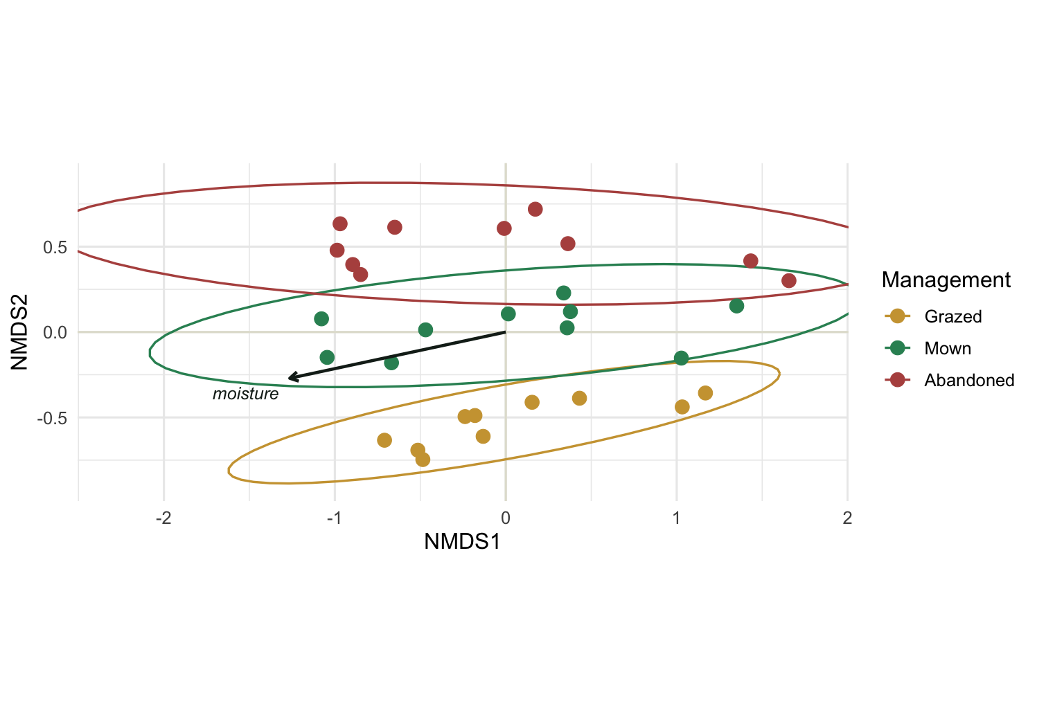
Two things are worth keeping in mind about envfit. A vector arrow assumes the variable changes smoothly and roughly linearly across the ordination plane. When a variable instead peaks in the middle and falls off at both ends, a straight arrow misrepresents it, and ordisurf() is the better tool: it drapes a fitted smooth surface over the ordination instead of a single direction. And a significant envfit result describes alignment with an existing picture, not a formal model of composition. For the latter, the next function is the one you want.
A third point follows from those two. envfit describes the ordination axes it was handed and nothing else: the r-squared it reports is the multiple R-squared of the variable regressed on those axes, and the axes it takes by default are the first two. The ordination here is two-dimensional, so that default sees everything there is; but when you keep more axes, a variable whose signal lies off the first plane can come back with a short, non-significant arrow while the community responds to it perfectly well. choices is the lever: passing choices = 1:k scores the variable against the first k axes rather than against the picture you happen to be plotting. And if the question is about the community rather than about the picture, the test belongs on the dissimilarity matrix itself, which is where the next function works.
PERMANOVA with adonis2: do the groups really differ?
Seeing three ellipses stack up is suggestive, but eyes find groups in noise. adonis2() runs PERMANOVA, which partitions the dissimilarity matrix among the predictors and asks, by reshuffling group labels many times, whether each predictor explains more of the total composition than random labelling would.
set.seed(42)
adonis2(vegdist(comm, "bray") ~ mgmt + moisture + pH,
        data = env, permutations = 999, by = "terms")
Permutation test for adonis under reduced model
Terms added sequentially (first to last)
Permutation: free
Number of permutations: 999
adonis2(formula = vegdist(comm, "bray") ~ mgmt + moisture + pH, data = env, permutations = 999, by = "terms")
Df SumOfSqs R2 F Pr(>F)
mgmt 2 1.4106 0.22436 9.0308 0.001 ***
moisture 1 2.8622 0.45524 36.6484 0.001 ***
pH 1 0.0620 0.00986 0.7940 0.501
Residual 25 1.9525 0.31054
Total 29 6.2874 1.00000
---
Signif. codes: 0 '***' 0.001 '**' 0.01 '*' 0.05 '.' 0.1 ' ' 1Each row carries a pseudo-F, an R-squared, and a permutation p-value. The R-squared is the share of the total multivariate variation that the term accounts for. Moisture takes the largest share, management a solid further chunk, and pH almost nothing, with a large p-value to match. The residual line is the variation left unexplained.
One detail decides how you read the table. by = "terms" adds the predictors in order, so each is tested on what is left after the ones above it. by = "margin" instead tests each predictor with all the others already accounted for. When predictors are independent, as moisture and management are here by construction, the two versions agree closely. When predictors are correlated, they can disagree sharply, and the order you wrote the formula in starts to change the story. Reaching for by = "margin" is the safer habit whenever you are unsure.
The p-values come from shuffling plots freely among the groups, and that assumes the plots are exchangeable: independent units, with no blocks, repeated visits or spatial pairing between them. That holds here by construction. If your plots are nested in sites or revisited over the years, free shuffling ignores that structure and the p-value is usually too small; restrict the permutations to match the design, as Repeated-measures PERMANOVA shows.
betadisper: is the difference real, or just uneven spread?
PERMANOVA has a trap that catches a lot of published work. It can return a significant result not because the group centroids sit in different places, but because the groups differ in how spread out they are internally. A tight cluster and a diffuse cloud can test as significantly different even with the same centre. betadisper() measures each plot’s distance to the centre of its own group and tests whether that spread differs between groups. By default the centre is the spatial median, not the centroid; type = "centroid" switches to the centroid.
bd <- betadisper(vegdist(comm, "bray"), mgmt)
set.seed(42)
permutest(bd, permutations = 999)
Permutation test for homogeneity of multivariate dispersions
Permutation: free
Number of permutations: 999

Response: Distances
          Df  Sum Sq  Mean Sq      F N.Perm Pr(>F)
Groups     2 0.05701 0.028504 0.9162    999  0.401
Residuals 27 0.84001 0.031112 data.frame(mgmt = mgmt, dist = bd$distances) %>%
ggplot(aes(mgmt, dist, fill = mgmt)) +
geom_boxplot(width = 0.55, outlier.shape = NA, alpha = 0.85) +
geom_jitter(width = 0.12, size = 1.6, color = "#2c3a31") +
scale_fill_manual(values = mgmt_cols, guide = "none") +
labs(x = NULL, y = "Distance to group median") +
theme_te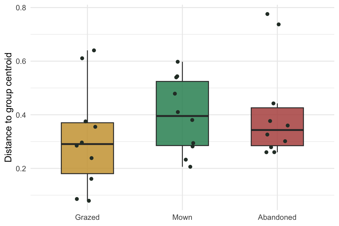
The test comes back non-significant (p around 0.4). In the box plot the grazed plots sit a little closer to their median than the other two groups; the mean distance to the group median runs from 0.31 to 0.41 across the three groups, a gap the test cannot tell apart from chance. That is not proof that the spreads are equal: a dispersion test can miss a modest difference, especially when the groups are small or unequal in size, as betadisper with unequal group sizes measures. What it does show is no sign of the uneven spread that would make the PERMANOVA ambiguous, and with equal group sizes, as here, PERMANOVA is fairly tolerant of a difference the test might have missed. That the management effect is a genuine difference in where the groups sit, and not an artefact of one regime being more variable, we know for certain only because the data were simulated that way; with field data it remains an inference. Had betadisper() been significant, the PERMANOVA p-value would have been unsafe to read as a centroid difference, and you would say so rather than quietly report the F-test. Running the two together, and reporting both, is the honest minimum.
Where to go next
The three functions form a small workflow: envfit() to see which gradients align with the map, adonis2() to test whether groupings explain composition, and betadisper() to make sure that test means what you think. From here, a pairwise PERMANOVA tells you which specific managements differ rather than just that some do; ordisurf() handles variables whose response curves bend; and constrained methods such as distance-based RDA (capscale() and dbrda()) let you model composition directly against predictors instead of fitting them onto an unconstrained map after the fact.
References
Anderson MJ 2001 Austral Ecology 26(1):32-46 (10.1111/j.1442-9993.2001.01070.pp.x)
McArdle BH, Anderson MJ 2001 Ecology 82(1):290-297 (10.1890/0012-9658(2001)082[0290:FMMTCD]2.0.CO;2)
Anderson MJ 2006 Biometrics 62(1):245-253 (10.1111/j.1541-0420.2005.00440.x)