library(ggplot2)
library(patchwork)
library(vegan)

te_paper  <- "#f5f4ee"
te_ink    <- "#16241d"
te_body   <- "#2c3a31"
te_forest <- "#275139"
te_rust   <- "#b5534e"
te_gold   <- "#c9b458"
te_line   <- "#dad9ca"

theme_datasheet <- function() {
  theme_minimal(base_size = 12) +
    theme(plot.background  = element_rect(fill = te_paper, colour = NA),
          panel.background = element_rect(fill = te_paper, colour = NA),
          panel.grid.major = element_line(colour = te_line, linewidth = 0.3),
          panel.grid.minor = element_blank(),
          text             = element_text(colour = te_body),
          plot.title       = element_text(colour = te_ink, face = "bold"),
          plot.subtitle    = element_text(colour = te_body),
          axis.text        = element_text(colour = te_body))
}Repeated-measures PERMANOVA in R: what to permute
R
vegan
PERMANOVA
permutation tests
repeated measures
experimental design
multivariate
simulation
ecology tutorial
Repeated-measures or paired PERMANOVA in R: shuffle whole sites to test a site-level treatment, within sites to test time. Free shuffling errs both ways.
Ten grassland sites, five grazed and five ungrazed, and the same quadrat at each site surveyed for vascular plants in four consecutive summers. Forty community samples go into one Bray-Curtis matrix and one call to adonis2(), with two questions for it: does grazing change composition, and does composition change over the four years? The samples are not forty independent units. Every site contributes four of them, and four samples from one site resemble each other more than they resemble samples from other sites. A permutation test gets its p-value by shuffling, so the question that decides whether the p-value means anything is what may be shuffled with what.
The short answer is that it depends on the term, and the two terms of this design need opposite schemes. Grazing is a property of the site: it is constant across the four years of a site, so the units that carry it are the ten sites, and the test has to exchange whole sites, keeping each site’s four samples together. Year varies inside every site, so its test has to shuffle the four samples within each site and never move a sample to another site. In the permute package these are how(within = Within(type = "none"), plots = Plots(strata = site, type = "free")) and how(blocks = site). The paired before/after design is the same problem with two visits per site. Free permutation, the adonis2() default, is wrong for both terms, in opposite directions: at the design simulated below it rejects a true null for grazing in most data sets and almost never rejects year, even when year has a real effect.
The post on common PERMANOVA mistakes names this as its Mistake 3, ignoring the design when permuting, and gives how(blocks = site) as the fix for subplots nested in sites. This post measures the two directions separately and adds the case its example does not cover, a site-level treatment, where the same blocking call returns p = 1 on every data set. Split-plot designs in ecology measured the same two opposite errors for a univariate ANOVA with one pooled residual, a whole-plot treatment too liberal and a subplot treatment too strict. Here the cause is the reference distribution rather than the error term, and the expected mean squares behind it are the same. Permutation tests from scratch keeps to unrestricted shuffling and says in its honest limits that the choice of what may be exchanged is “a larger source of error than anything measured above”; this is that choice for the commonest ecological design with structure. And pairwise PERMANOVA loops adonis2() over pairs of groups with free permutations, which a repeated-measures study would have to restrict in the same way inside every pair.
None of the logic is new. PERMANOVA is Anderson 2001, and Anderson and ter Braak 2003 gave a guideline for building an exact permutation test, where one exists, for any term of an analysis-of-variance design, and their simulations showed that the choice of units exchangeable under the null hypothesis is essential for every test, whether exact or approximate. For the two terms here the guideline comes down to permuting the units at the level where the term varies. What follows is a demonstration of that rule on community data, with the size of each error measured.
Forty samples from ten sites
The simulated communities have 30 species. Each species has a mean log abundance drawn once per data set, each site shifts every species by its own normal deviation with standard deviation 0.8, and each sample adds independent noise with standard deviation 0.3 before a Poisson draw. The site deviations are what make four samples from one site alike. When a year effect is switched on, the first 8 species change their log abundance by 0.25 per year; when a grazing effect is switched on, 8 other species are shifted by 1 in the grazed sites. All of these constants were fixed before the simulations below were run.
n_sp <- 30
make_design <- function(n_site, n_year) {
  des <- data.frame(site = factor(rep(seq_len(n_site), each = n_year)),
                    year = factor(rep(seq_len(n_year), n_site)))
  des$treat <- factor(ifelse(as.integer(des$site) <= n_site / 2, "ungrazed", "grazed"))
  des
}
sim_comm <- function(des, site_sd, year_eff, treat_eff, noise_sd = 0.3) {
  n <- nrow(des); n_s <- nlevels(des$site)
  mu0 <- rnorm(n_sp, 1.5, 1)
  site_dev <- matrix(rnorm(n_s * n_sp, 0, site_sd), n_s, n_sp)
  yr_score <- as.integer(des$year) - mean(seq_len(nlevels(des$year)))
  eta <- matrix(mu0, n, n_sp, byrow = TRUE) + site_dev[as.integer(des$site), ] +
    outer(yr_score, c(rep(year_eff, 8), rep(0, n_sp - 8))) +
    outer(des$treat == "grazed", c(rep(0, 8), rep(treat_eff, 8), rep(0, n_sp - 16))) +
    matrix(rnorm(n * n_sp, 0, noise_sd), n, n_sp)
  Y <- matrix(rpois(n * n_sp, exp(eta)), n, n_sp)
  Y[rowSums(Y) == 0, 1] <- 1
  Y
}
des40 <- make_design(10, 4)
The simulations need thousands of PERMANOVAs, so they use a base R version of the statistic. McArdle and Anderson 2001 write the pseudo-F as a ratio of traces: square the dissimilarities, multiply by minus a half and centre the rows and columns (Gower centring) to get a matrix \(G\); a term’s sum of squares is then \(\mathrm{tr}(A G)\), where \(A\) is the difference between the projection matrices of the model with and without the term, and the residual sum of squares is \(\mathrm{tr}(G)\) minus the trace of the full model’s projection times \(G\). Shuffling the samples by a permutation \(P\) replaces \(G\) with \(P G P^{\top}\), which is the same as moving the rows of an orthonormal basis of \(A\), so a whole set of permutations costs one matrix product.
bray_base <- function(Y) {
  n <- nrow(Y); num <- matrix(0, n, n)
  for (k in seq_len(ncol(Y))) num <- num + abs(outer(Y[, k], Y[, k], "-"))
  tot <- rowSums(Y)
  num / outer(tot, tot, "+")
}
gower_centre <- function(D) {
  A <- -0.5 * D^2
  A <- sweep(A, 1, rowMeans(A))
  sweep(A, 2, colMeans(A))
}
proj <- function(X) X %*% solve(crossprod(X), t(X))
orth <- function(M) { e <- eigen(M, symmetric = TRUE); e$vectors[, e$values > 0.5, drop = FALSE] }
term_form <- function(des, small, big) {        # the term 'big' minus 'small', and the residual of 'big'
  Xs <- model.matrix(as.formula(paste("~", small)), des)
  Xb <- model.matrix(as.formula(paste("~", big)), des)
  n <- nrow(des)
  list(QA = orth(proj(Xb) - proj(Xs)), QB = orth(proj(Xb) - matrix(1 / n, n, n)),
       df1 = ncol(Xb) - ncol(Xs), df2 = n - ncol(Xb))
}
ss_perm <- function(G, Q, P) {                    # tr(Q' G Q) after each permutation (row of P)
  B <- nrow(P); n <- ncol(P); k <- ncol(Q)
  Qp <- matrix(array(Q[as.vector(t(P)), ], c(n, B, k)), n)
  rowSums(matrix(colSums(Qp * (G %*% Qp)), B, k))
}
f_perm <- function(G, fm, P) {
  (ss_perm(G, fm$QA, P) / fm$df1) / ((sum(diag(G)) - ss_perm(G, fm$QB, P)) / fm$df2)
}
f_obs <- function(G, fm) f_perm(G, fm, matrix(seq_len(nrow(G)), 1))
p_of <- function(G, fm, P) (1 + sum(f_perm(G, fm, P) >= f_obs(G, fm) - 1e-9)) / (1 + nrow(P))
forms_for <- function(des) list(
  treat = term_form(des, "1", "treat"), year = term_form(des, "1", "year"),
  year_site = term_form(des, "site", "site + year"), site = term_form(des, "1", "site"))
fm40 <- forms_for(des40)

set.seed(33401)
Y_field <- sim_comm(des40, site_sd = 0.8, year_eff = 0.25, treat_eff = 0)
G_field <- gower_centre(bray_base(Y_field))
f_check <- rbind(
  base_r  = c(treat = f_obs(G_field, fm40$treat), year = f_obs(G_field, fm40$year),
              year_after_site = f_obs(G_field, fm40$year_site)),
  adonis2 = c(adonis2(Y_field ~ treat, data = des40, permutations = 0)$F[1],
              adonis2(Y_field ~ year, data = des40, permutations = 0)$F[1],
              adonis2(Y_field ~ site + year, data = des40, permutations = 0, by = "terms")$F[2]))
bray_gap <- max(abs(bray_base(Y_field) - as.matrix(vegdist(Y_field, "bray"))))
f_gap <- max(abs(f_check[1, ] - f_check[2, ]))
round(f_check, 4)
treat year year_after_site
base_r 4.6157 0.3713 1.8881
adonis2 4.6157 0.3713 1.8881On one simulated field data set, with a year effect and no grazing effect, the base R Bray-Curtis matrix matches vegdist() exactly and the three pseudo-F values (grazing alone, year alone, year after site) agree with adonis2() to within floating-point rounding. Everything below that uses the base R statistic is therefore the adonis2() statistic; only the shuffling differs.
Three ways to shuffle forty samples
Free permutation treats all forty samples as exchangeable. Shuffling within sites keeps every sample at its own site and reorders the four years inside each one. Shuffling whole sites moves each site’s four samples as a unit to another site’s four slots, keeping their year order. The chunk below builds each kind for the base R machinery, then asks the permute package for the two restricted schemes and for a third call, the bare Plots(strata = site).
perm_sets <- function(des, B) {
  n <- nrow(des); s <- as.integer(des$site); n_s <- max(s); n_y <- n / n_s
  b <- rep(seq_len(B), each = n)
  free <- matrix(order(b, runif(B * n)) - (b - 1) * n, B, byrow = TRUE)
  within <- matrix(order(b, rep(s, B), runif(B * n)) - (b - 1) * n, B, byrow = TRUE)
  bs <- rep(seq_len(B), each = n_s)
  site_order <- matrix(order(bs, runif(B * n_s)) - (bs - 1) * n_s, B, byrow = TRUE)
  whole <- (site_order[, rep(seq_len(n_s), each = n_y)] - 1) * n_y +
    matrix(rep(seq_len(n_y), n_s), B, n, byrow = TRUE)
  list(free = free, within = within, whole = whole)
}

library(permute)
site <- des40$site
ctrl_within <- how(blocks = site)
ctrl_whole  <- how(within = Within(type = "none"), plots = Plots(strata = site, type = "free"))
ctrl_plots_default <- how(plots = Plots(strata = site))
set.seed(33402)
one_each <- rbind(within = shuffleSet(40, 1, control = ctrl_within)[1, ],
                  whole = shuffleSet(40, 1, control = ctrl_whole)[1, ],
                  plots_default = shuffleSet(40, 1, control = ctrl_plots_default)[1, ])
stays_home <- apply(one_each, 1, function(p) all(site[p] == site))
one_each[, 1:12]
[,1] [,2] [,3] [,4] [,5] [,6] [,7] [,8] [,9] [,10] [,11] [,12]
within 3 2 4 1 8 5 7 6 10 11 9 12
whole 29 30 31 32 25 26 27 28 37 38 39 40
plots_default 1 2 3 4 8 7 6 5 12 9 10 11stays_home within whole plots_default
TRUE FALSE TRUE The third call is the one to watch. Plots(strata = site) on its own declares the sites as plots but leaves the plots themselves unshuffled (the default type = "none") and shuffles freely inside each one (the default Within()), so it is another way of writing the within-site scheme: in the draw above every sample stays at its home site under both how(blocks = site) and the bare Plots() call (within = TRUE, whole = FALSE, plots_default = TRUE). Exchanging whole sites needs both arguments spelled out, Within(type = "none") so the four samples keep their order and type = "free" on the plots so the sites move; for the grazing test only type = "free" matters, since reordering years inside a site leaves the grazing sum of squares unchanged.
set.seed(33403)
draw1 <- lapply(perm_sets(des40, 1), function(p) p[1, ])
tile_df <- do.call(rbind, lapply(names(draw1), function(nm) {
  p <- draw1[[nm]]
  data.frame(scheme = nm, slot_site = as.integer(des40$site), slot_year = as.integer(des40$year),
             from_site = as.integer(des40$site)[p], from_year = as.integer(des40$year)[p])
}))
tile_df$home <- ifelse(tile_df$from_site == tile_df$slot_site, "own site", "another site")
tile_df$scheme <- factor(c(free = "free", within = "within sites", whole = "whole sites")[tile_df$scheme],
                         levels = c("free", "within sites", "whole sites"))
ggplot(tile_df, aes(slot_year, slot_site, fill = home)) +
  geom_tile(colour = te_paper, linewidth = 0.8) +
  geom_text(aes(label = from_site), colour = te_paper, size = 3.2, fontface = "bold") +
  facet_wrap(~ scheme) +
  scale_y_reverse(breaks = 1:10) +
  scale_x_continuous(breaks = 1:4) +
  scale_fill_manual(values = c("own site" = te_forest, "another site" = te_rust), name = NULL) +
  labs(x = "year slot", y = "site slot", title = "Where one shuffle puts each sample") +
  theme_datasheet() +
  theme(panel.grid.major = element_blank(), legend.position = "bottom",
        strip.text = element_text(colour = te_ink, face = "bold"))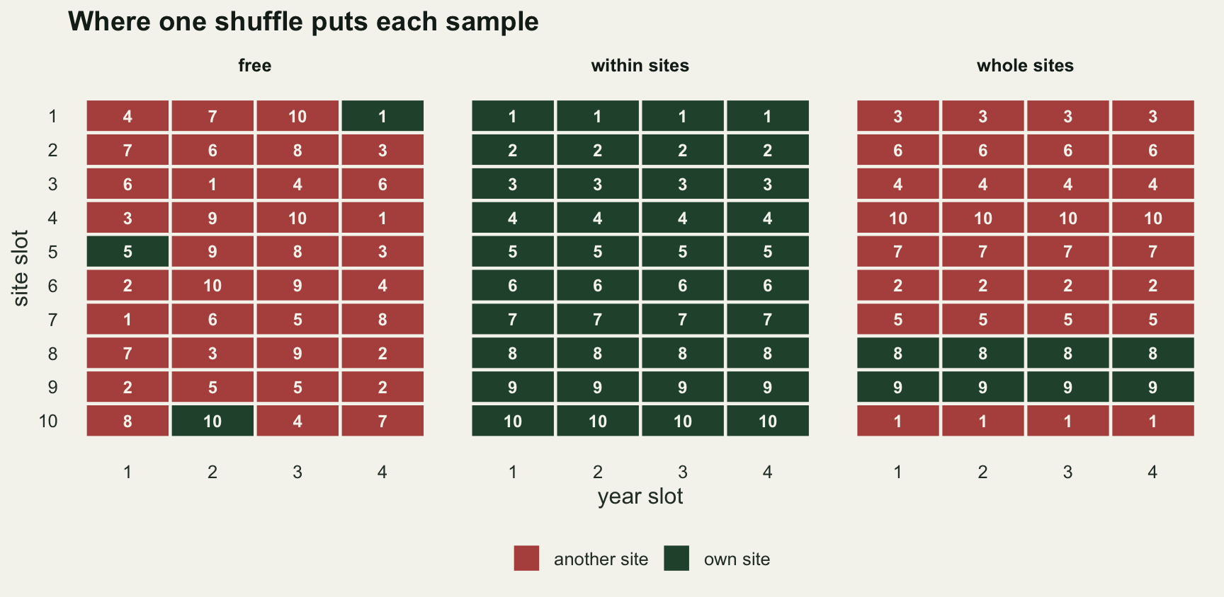
A label the shuffle cannot move
The blocking call that fixes Mistake 3 in the neighbour post is right for year and useless for grazing. Grazing is constant within every site, so a permutation that keeps each sample at its own site leaves every sample with the grazing label it started with. Every permuted data set pairs each sample with the grazing label it already had, every permuted pseudo-F equals the observed one, and the p-value, the share of permuted values at least as large as the observed, is 1. The same happens in mirror image when whole sites are exchanged and year is tested: the sites move with their year order intact, so each sample keeps its year.
p_table <- function(Y, des, ctrl_list, seed) {
  sapply(c("treat", "year"), function(term) sapply(names(ctrl_list), function(nm) {
    set.seed(seed)
    adonis2(as.formula(paste("Y ~", term)), data = des, permutations = ctrl_list[[nm]])$`Pr(>F)`[1]
  }))
}
ctrl_999 <- list(free = how(nperm = 999),
                 within_sites = how(blocks = site, nperm = 999),
                 whole_sites = how(within = Within(type = "none"), plots = Plots(strata = site, type = "free"),
                                   nperm = 999),
                 plots_default = how(plots = Plots(strata = site), nperm = 999))
trap_p <- p_table(Y_field, des40, ctrl_999, 33404)
set.seed(33404)
p_strata_arg <- adonis2(Y_field ~ treat, data = des40, permutations = 999, strata = site)$`Pr(>F)`[1]
set.seed(33405)
ps_demo <- perm_sets(des40, 999)
spread <- c(treat_within = diff(range(f_perm(G_field, fm40$treat, ps_demo$within))),
            year_whole = diff(range(f_perm(G_field, fm40$year, ps_demo$whole))))
set.seed(33404)
fit_blocked_treat <- adonis2(Y_field ~ treat, data = des40, permutations = ctrl_999$within_sites)
set.seed(33404)
fit_free_year <- adonis2(Y_field ~ year, data = des40, permutations = ctrl_999$free)
spread_adonis <- c(treat_blocks = diff(range(permustats(fit_blocked_treat)$permutations)),
                   year_free = diff(range(permustats(fit_free_year)$permutations)))
trap_p
treat year
free 0.001 1.000
within_sites 1.000 0.006
whole_sites 0.250 1.000
plots_default 1.000 0.005c(strata_argument = p_strata_arg)strata_argument
1 spreadtreat_within year_whole
1.776357e-15 6.661338e-16 spread_adonistreat_blocks year_free
2.664535e-15 2.376957e+00 On the field data set adonis2() gives grazing a p-value of 1.000 under how(blocks = site) and 1.000 under the bare Plots(strata = site) call, 1.000 with the older strata = site argument of adonis2() (which vegan turns into the same blocks), and year 1.000 under whole-site shuffling. The base R version shows why: across 999 within-site permutations the grazing pseudo-F has a spread (largest minus smallest) of zero up to floating-point rounding, and across 999 whole-site permutations so does the year pseudo-F (both spreads are printed above). A p-value of exactly 1 together with a permutation distribution of zero spread is the signature of a term tested with a scheme that cannot move it; it is not evidence of no effect. A p of 1 on its own is not that signature. Free permutation gives year 1.000 on this same data set because nearly all of a widely spread null lies above the observed value; that is the opposite failure, a test held too strict, and the main simulation below finds a free-permutation p of exactly 1 for year in most of its null data sets. adonis2() keeps its permuted pseudo-F values, so telling the two apart takes one line, diff(range(permustats(fit)$permutations)): it returns zero up to floating-point rounding for grazing under how(blocks = site) (the value printed above) and 2.38 for year under free permutation.
The two schemes that can move each label give grazing 0.250 (whole sites) against 0.001 (free), and year 0.006 (within sites) against 1.000 (free). This data set has a real year effect and no grazing effect. One data set shows what the output looks like; the rates follow further down.
Where each null is centred
Why free permutation errs, and in which direction, is arithmetic. Take a term whose sum of squares is \(\mathrm{tr}(A G)\), with \(A\) of rank \(q\) and centred. Averaged over all permutations of the forty samples, \(P G P^{\top}\) becomes \(\mathrm{tr}(G)/(n-1)\) times the centring matrix, so the permuted sum of squares averages \(q \, \mathrm{tr}(G)/(n-1)\): the free null puts the term’s mean square, on average, at the total mean square \(\mathrm{MS}_{\text{total}}\). The same argument, applied to the site means, puts the average of a between-site term under whole-site shuffling at the between-site mean square \(\mathrm{MS}_{\text{site}}\), and applied inside the sites, it puts a within-site term under within-site shuffling at the within-site mean square \(\mathrm{MS}_{\text{within}}\). These are the two strata of the split-plot post, read off a dissimilarity matrix.
Under the null the observed grazing mean square has the expectation of \(\mathrm{MS}_{\text{site}}\), since grazing is one more way of grouping sites, and the observed year mean square has the expectation of \(\mathrm{MS}_{\text{within}}\), since in a balanced design every year contains every site and the site differences cancel. The total mean square is a weighted average of the two strata, \(\left[(s - 1)\mathrm{MS}_{\text{site}} + (n - s)\mathrm{MS}_{\text{within}}\right]/(n - 1)\) for \(s\) sites, so whenever the between-site mean square exceeds the within-site one, it sits below the first and above the second. Free permutation centres both nulls there: too low for grazing, which then looks large, and too high for year, which then looks small. In a one-term model the pseudo-F is an increasing function of the term’s sum of squares (the total is fixed), so where the sum of squares falls in the null decides the p-value.
set.seed(33406)
Y_null <- sim_comm(des40, site_sd = 0.8, year_eff = 0, treat_eff = 0)
G_null <- gower_centre(bray_base(Y_null))
ms_strata <- function(G, fm) {
  tot <- sum(diag(G)); n <- nrow(G); s_df <- fm$site$df1
  ss_s <- ss_perm(G, fm$site$QA, matrix(seq_len(n), 1))
  c(site = ss_s / s_df, within = (tot - ss_s) / (n - 1 - s_df), total = tot / (n - 1))
}
ms0 <- ms_strata(G_null, fm40)
ps_big <- perm_sets(des40, 4999)
id1 <- matrix(seq_len(40), 1)
ms_term <- function(Q, df1, P) ss_perm(G_null, Q, P) / df1
centre_tab <- rbind(
  treat = c(observed = ms_term(fm40$treat$QA, 1, id1),
            free_mean = mean(ms_term(fm40$treat$QA, 1, ps_big$free)),
            restricted_mean = mean(ms_term(fm40$treat$QA, 1, ps_big$whole)),
            predicted_free = ms0[["total"]], predicted_restricted = ms0[["site"]]),
  year = c(observed = ms_term(fm40$year$QA, 3, id1),
           free_mean = mean(ms_term(fm40$year$QA, 3, ps_big$free)),
           restricted_mean = mean(ms_term(fm40$year$QA, 3, ps_big$within)),
           predicted_free = ms0[["total"]], predicted_restricted = ms0[["within"]]))
centre_gap <- max(abs(centre_tab[, c("free_mean", "restricted_mean")] /
                        centre_tab[, c("predicted_free", "predicted_restricted")] - 1))
site_F0 <- f_obs(G_null, fm40$site)
null_f <- list(treat_free = f_perm(G_null, fm40$treat, ps_big$free), treat_whole = f_perm(G_null, fm40$treat, ps_big$whole),
               year_free = f_perm(G_null, fm40$year, ps_big$free), year_within = f_perm(G_null, fm40$year, ps_big$within))
obs_f <- c(treat = f_obs(G_null, fm40$treat), year = f_obs(G_null, fm40$year))
p_null_demo <- c(treat_free = mean(c(null_f$treat_free, obs_f[["treat"]]) >= obs_f[["treat"]] - 1e-9),
                 treat_whole = mean(c(null_f$treat_whole, obs_f[["treat"]]) >= obs_f[["treat"]] - 1e-9),
                 year_free = mean(c(null_f$year_free, obs_f[["year"]]) >= obs_f[["year"]] - 1e-9),
                 year_within = mean(c(null_f$year_within, obs_f[["year"]]) >= obs_f[["year"]] - 1e-9))
signif(ms0, 3)
site within total
0.3790 0.0254 0.1070 signif(centre_tab, 3) observed free_mean restricted_mean predicted_free predicted_restricted
treat 0.5350 0.107 0.3820 0.107 0.3790
year 0.0192 0.108 0.0253 0.107 0.0254round(c(site_F = site_F0, p_null_demo), 4) site_F treat_free treat_whole year_free year_within
14.9533 0.0002 0.1226 1.0000 0.8448 On a data set with no grazing effect and no year effect, the between-site mean square is 0.3792, the within-site one 0.0254 and the total 0.1070. Over 4999 permutations of each kind the four permutation means land within 0.6 per cent of the predicted stratum. The observed grazing mean square, 0.5354, is compared by free permutation with a null centred at 0.1066; the observed year mean square, 0.0192, with the same kind of null centred at 0.1075.
null_df <- rbind(
  data.frame(term = "grazing (between sites)", scheme = "free", f = null_f$treat_free),
  data.frame(term = "grazing (between sites)", scheme = "design-based", f = null_f$treat_whole),
  data.frame(term = "year (within sites)", scheme = "free", f = null_f$year_free),
  data.frame(term = "year (within sites)", scheme = "design-based", f = null_f$year_within))
null_df$scheme <- factor(null_df$scheme, levels = c("free", "design-based"))
obs_df <- data.frame(term = c("grazing (between sites)", "year (within sites)"), f = obs_f)
null_plot <- function(tm, ttl) {
  ggplot(null_df[null_df$term == tm, ], aes(f, fill = scheme)) +
    geom_histogram(bins = 60, position = "identity", alpha = 0.6, colour = NA) +
    geom_vline(data = obs_df[obs_df$term == tm, ], aes(xintercept = f), colour = te_ink,
               linetype = "dashed", linewidth = 0.6) +
    scale_fill_manual(values = c(free = te_rust, "design-based" = te_forest), name = NULL) +
    labs(x = "pseudo-F", y = "permutations", title = ttl) +
    theme_datasheet() +
    theme(legend.position = "bottom", plot.title = element_text(size = 11, colour = te_ink, face = "bold"))
}
null_plot("grazing (between sites)", "Grazing: free vs whole sites") +
  null_plot("year (within sites)", "Year: free vs within sites") +
  plot_annotation(theme = theme_datasheet())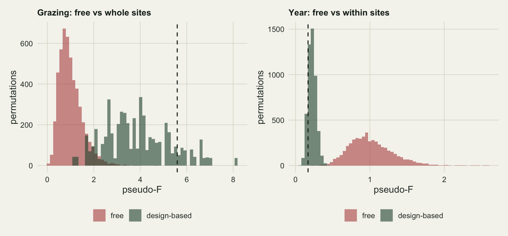
The observed grazing pseudo-F, 5.59, is equalled or exceeded by a share of 0.0002 of the free null, counting the observed value itself, and by 0.123 of the whole-site null. The observed year pseudo-F, 0.168, is equalled or exceeded by 1.000 of the free null and 0.845 of the within-site one. These shares are the permutation p-values for this data set. The ratio that sets how far apart the strata are is \(\mathrm{MS}_{\text{site}}/\mathrm{MS}_{\text{within}}\), which is exactly the pseudo-F of adonis2(D ~ site); here it is 15.0.
Size and power at ten sites and four years
The main simulation runs 1000 data sets with no effect of either term, 600 with a grazing effect only and 600 with a year effect only, at the design above: 10 sites, 5 of them grazed, 4 years, site standard deviation 0.8. Each test uses 199 random permutations and rejects at p at most 0.05, which with 200 values including the observed one gives a level of at most five per cent when the scheme is right (exactly five without tied values). Eight tests run on every data set: grazing under the three schemes, year under the three schemes, and year after site (D ~ site + year) under free and within-site permutation, the model-based alternative taken up below.
one_rep <- function(des, fm, site_sd, year_eff, treat_eff, B = 199) {
  G <- gower_centre(bray_base(sim_comm(des, site_sd, year_eff, treat_eff)))
  ps <- perm_sets(des, B)
  c(treat_free = p_of(G, fm$treat, ps$free), treat_within = p_of(G, fm$treat, ps$within),
    treat_whole = p_of(G, fm$treat, ps$whole),
    year_free = p_of(G, fm$year, ps$free), year_within = p_of(G, fm$year, ps$within),
    year_whole = p_of(G, fm$year, ps$whole), year_site_free = p_of(G, fm$year_site, ps$free),
    year_site_within = p_of(G, fm$year_site, ps$within), site_F = f_obs(G, fm$site))
}
run_cond <- function(des, fm, n_rep, site_sd, year_eff, treat_eff, seed) {
  set.seed(seed)
  t(replicate(n_rep, one_rep(des, fm, site_sd, year_eff, treat_eff)))
}
rate_of <- function(res) colMeans(res[, colnames(res) != "site_F"] <= 0.05)
mc_se <- function(p, n_rep) sqrt(p * (1 - p) / n_rep)
n_null <- 1000; n_eff <- 600
res_null <- run_cond(des40, fm40, n_null, 0.8, 0, 0, 33410)
res_treat <- run_cond(des40, fm40, n_eff, 0.8, 0, 1, 33411)
res_year <- run_cond(des40, fm40, n_eff, 0.8, 0.25, 0, 33412)
rates <- rbind(size = rate_of(res_null), power_treat = rate_of(res_treat), power_year = rate_of(res_year))
se_size <- mc_se(0.05, n_null)
same_p_blocked <- all(res_null[, "year_within"] == res_null[, "year_site_within"]) &&
all(res_year[, "year_within"] == res_year[, "year_site_within"])
thesis_dead <- rates["size", "treat_free"] < 0.15 &&
abs(rates["power_year", "year_free"] - rates["power_year", "year_within"]) < 0.10
trap_all_one <- all(c(res_null[, "treat_within"], res_treat[, "treat_within"],
res_null[, "year_whole"], res_year[, "year_whole"]) == 1)
p1_year_free <- c(null = mean(res_null[, "year_free"] == 1), effect = mean(res_year[, "year_free"] == 1))
r3 <- function(x) sprintf("%.3f", x)
se3 <- function(p, n_rep) sprintf("%.3f", mc_se(p, n_rep))
round(rates, 3) treat_free treat_within treat_whole year_free year_within
size 0.911 0 0.045 0 0.048
power_treat 1.000 0 0.587 0 0.018
power_year 0.925 0 0.052 0 0.902
year_whole year_site_free year_site_within
size 0 0.024 0.048
power_treat 0 0.007 0.018
power_year 0 0.847 0.902c(mc_se_at_0.05 = round(se_size, 4), same_p_blocked = same_p_blocked, trap_all_one = trap_all_one,
thesis_dead = thesis_dead) mc_se_at_0.05 same_p_blocked trap_all_one thesis_dead
0.0069 1.0000 1.0000 0.0000 round(p1_year_free, 3) null effect
0.975 0.245 Grazing first. Free permutation rejects the true null in 0.911 of the data sets (Monte Carlo standard error 0.009): a PERMANOVA that ignores the sites reports a grazing effect in most of these simulated studies, none of which has one. Whole-site shuffling rejects 0.045 (standard error 0.007 at the nominal level), and when grazing does shift 8 species it detects it in 0.587 of the data sets (standard error 0.020). The test compares five grazed sites with five ungrazed ones, so its replication is ten sites, not forty samples; treating the forty as replicates is the multivariate form of pseudoreplication. Within-site shuffling rejects grazing in 0.000 of the null data sets and 0.000 of those with an effect: its p-value was exactly 1 on every draw, the trap described above.
Year goes the other way. Free permutation with D ~ year rejects a true null in 0.000 of data sets, which could pass for caution, and detects the real year effect in 0.000 of the data sets that have one. Its p-value is exactly 1 in 0.975 of the null data sets and 0.245 of those with a year effect, from a null that is spread out rather than stuck, so a p of 1 by itself does not identify the trap. Within-site shuffling holds its size at 0.048 and detects the effect in 0.902 (standard error 0.012). Whole-site shuffling rejects year in 0.000 and 0.000, the mirror trap, again with p = 1 on every draw.
Adding site to the model does not change the within-site test at all: with D ~ site + year and within-site shuffling the p-values are identical to those of D ~ year on all 1600 null and year-effect data sets, because within-site shuffling leaves the site sum of squares fixed and the year pseudo-F is then a monotone function of the year sum of squares in both models. Site in the model changes the pseudo-F and R squared that get reported, not the p-value.
With site in the model, free permutation of the raw samples becomes nearly usable for year. Anderson and Legendre 1999 compared permuting raw data with permuting residuals for partial tests, and a free shuffle of raw data with the nuisance term in the model is one of the approximate schemes they studied; Permutation tests with a covariate in the model measures it for a continuous covariate. Here it rejects a true null in 0.024 of data sets (standard error 0.007 at the nominal level) and detects the year effect in 0.847, against 0.902 for within-site shuffling. It is conservative and it costs power, and it cannot test grazing, which is aliased with site. Within-site shuffling is exact and no harder to write.
Before and after at the same sites
The paired design is the same problem with two visits. Ten sites are surveyed once before and once after an event, and the question is whether composition changed; there is no between-site treatment. Within-site shuffling swaps or keeps the two samples of each site, which gives only \(2^{10} = 1024\) arrangements and, since swapping every pair returns the same pseudo-F, at most 512 distinct values, still enough for a five per cent test. The simulation runs 1000 data sets without an effect and 1000 with a step of 0.5 in log abundance for the first 8 species at the second visit.
des20 <- make_design(10, 2)
fm20 <- forms_for(des20)
res_pair0 <- run_cond(des20, fm20, 1000, 0.8, 0, 0, 33420)
res_pair1 <- run_cond(des20, fm20, 1000, 0.8, 0.5, 0, 33421)
cols_pair <- c("year_free", "year_within", "year_site_free", "year_whole")
rates_pair <- rbind(size = rate_of(res_pair0)[cols_pair], power = rate_of(res_pair1)[cols_pair])
n_pair_perm <- numPerms(20, how(blocks = des20$site))
round(rates_pair, 3)
year_free year_within year_site_free year_whole
size 0.000 0.051 0.032 0
power 0.002 0.702 0.633 0n_pair_perm[1] 1024The pattern repeats. Free permutation with D ~ visit (the two-level year factor in the code) rejects in 0.000 of the null data sets and 0.002 of those with a change. Within-site shuffling gives 0.051 and 0.702 (standard errors 0.007 and 0.014). Free shuffling with site in the model gives 0.032 and 0.633. The permute package counts 1024 arrangements for how(blocks = site) at this design.
scheme_lab <- c(free = "free", within = "within sites", whole = "whole sites", site_free = "free, site in model")
rate_long <- function(r_null, r_eff, n0, n1, term, pref, keep) {
  do.call(rbind, lapply(keep, function(k) {
    cname <- paste(pref, k, sep = "_")
    data.frame(term = term, scheme = scheme_lab[[k]],
               what = c("no effect", "effect"), rate = c(r_null[[cname]], r_eff[[cname]]),
               se = c(mc_se(r_null[[cname]], n0), mc_se(r_eff[[cname]], n1)))
  }))
}
rates_df <- rbind(
  rate_long(rates["size", ], rates["power_treat", ], n_null, n_eff, "grazing, 10 sites x 4 years", "treat",
            c("free", "within", "whole")),
  rate_long(rates["size", ], rates["power_year", ], n_null, n_eff, "year, 10 sites x 4 years", "year",
            c("free", "within", "whole", "site_free")),
  rate_long(rates_pair["size", ], rates_pair["power", ], 1000, 1000, "before and after, 10 sites", "year",
            c("free", "within", "whole", "site_free")))
rates_df$term <- factor(rates_df$term, levels = unique(rates_df$term))
rates_df$scheme <- factor(rates_df$scheme, levels = rev(scheme_lab))
rates_df$what <- factor(rates_df$what, levels = c("no effect", "effect"))
p_rates <- ggplot(rates_df, aes(rate, scheme, colour = what, shape = what)) +
  geom_vline(xintercept = 0.05, colour = te_ink, linetype = "dashed", linewidth = 0.5) +
  geom_errorbar(aes(xmin = pmax(rate - 2 * se, 0), xmax = pmin(rate + 2 * se, 1)), orientation = "y",
                width = 0, linewidth = 0.6, position = position_dodge(width = 0.5)) +
  geom_point(size = 2.6, position = position_dodge(width = 0.5)) +
  facet_wrap(~ term, nrow = 1) +
  scale_x_continuous(limits = c(0, 1), breaks = c(0.05, 0.25, 0.5, 0.75, 1),
                     labels = c("0.05", "0.25", "0.5", "0.75", "1")) +
  scale_colour_manual(values = c("no effect" = te_rust, effect = te_forest), name = NULL) +
  scale_shape_manual(values = c("no effect" = 16, effect = 17), name = NULL) +
  labs(x = "rejection rate", y = NULL, title = "Each term has one scheme that works") +
  theme_datasheet() +
  theme(legend.position = "bottom", strip.text = element_text(colour = te_ink, face = "bold"),
        panel.spacing = unit(1.2, "lines"))
p_rates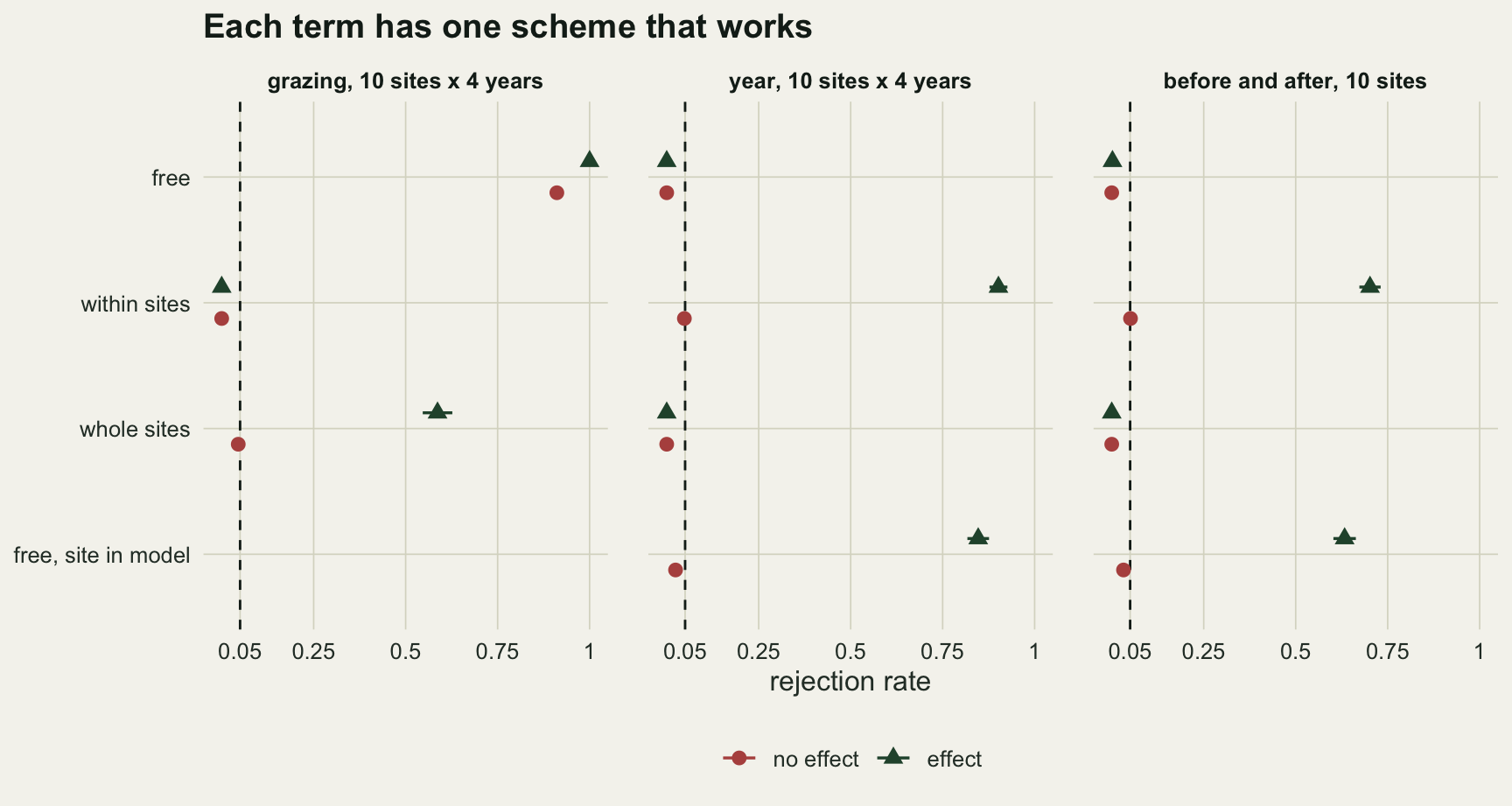
How much site variation it takes
Everything so far used one value for the spread among sites. The arithmetic says free permutation errs whenever \(\mathrm{MS}_{\text{site}}\) exceeds \(\mathrm{MS}_{\text{within}}\), and by more the further apart they are, so the last simulation varies the site standard deviation over 0, 0.2, 0.4, 0.8 and 1.2 (the 0.8 cell reuses the main runs) with 300 null and 300 year-effect data sets at each new value, and records the site pseudo-F of every data set.
sd_new <- c(0, 0.2, 0.4, 1.2)
sweep_one <- function(sd_site, k) {
  r0 <- run_cond(des40, fm40, 300, sd_site, 0, 0, 33430 + k)
  r1 <- run_cond(des40, fm40, 300, sd_site, 0.25, 0, 33440 + k)
  list(r0 = r0, r1 = r1)
}
sweep_runs <- lapply(seq_along(sd_new), function(k) sweep_one(sd_new[k], k))
sweep_row <- function(sd_site, r0, r1) {
  data.frame(site_sd = sd_site, n0 = nrow(r0), n1 = nrow(r1), site_F = median(r0[, "site_F"]),
             treat_free = mean(r0[, "treat_free"] <= 0.05), treat_whole = mean(r0[, "treat_whole"] <= 0.05),
             year_free_size = mean(r0[, "year_free"] <= 0.05), year_within_size = mean(r0[, "year_within"] <= 0.05),
             year_free_pow = mean(r1[, "year_free"] <= 0.05), year_within_pow = mean(r1[, "year_within"] <= 0.05),
             year_site_free_pow = mean(r1[, "year_site_free"] <= 0.05))
}
sweep_tab <- rbind(do.call(rbind, lapply(seq_along(sd_new), function(k)
                     sweep_row(sd_new[k], sweep_runs[[k]]$r0, sweep_runs[[k]]$r1))),
                   sweep_row(0.8, res_null, res_year))
sweep_tab <- sweep_tab[order(sweep_tab$site_sd), ]
sw <- function(sd_site, col) sweep_tab[[col]][sweep_tab$site_sd == sd_site]
z_design <- max(abs(c(sweep_tab$treat_whole, sweep_tab$year_within_size) - 0.05) /
                  mc_se(0.05, c(sweep_tab$n0, sweep_tab$n0)))
round(sweep_tab, 3)
site_sd n0 n1 site_F treat_free treat_whole year_free_size
1 0.0 300 300 0.999 0.053 0.047 0.04
2 0.2 300 300 1.791 0.360 0.040 0.00
3 0.4 300 300 4.267 0.740 0.023 0.00
5 0.8 1000 600 13.716 0.911 0.045 0.00
4 1.2 300 300 28.708 0.967 0.053 0.00
year_within_size year_free_pow year_within_pow year_site_free_pow
1 0.040 0.947 0.943 0.953
2 0.037 0.823 0.927 0.920
3 0.043 0.270 0.897 0.893
5 0.048 0.000 0.902 0.847
4 0.027 0.000 0.830 0.730sw_a <- rbind(data.frame(site_F = sweep_tab$site_F, rate = sweep_tab$treat_free, n = sweep_tab$n0, scheme = "free"),
data.frame(site_F = sweep_tab$site_F, rate = sweep_tab$treat_whole, n = sweep_tab$n0, scheme = "whole sites"))
sw_b <- rbind(data.frame(site_F = sweep_tab$site_F, rate = sweep_tab$year_free_pow, n = sweep_tab$n1, scheme = "free"),
data.frame(site_F = sweep_tab$site_F, rate = sweep_tab$year_within_pow, n = sweep_tab$n1, scheme = "within sites"),
data.frame(site_F = sweep_tab$site_F, rate = sweep_tab$year_site_free_pow, n = sweep_tab$n1,
scheme = "free, site in model"))
sweep_plot <- function(d, cols, ttl, ylab, ref = TRUE) {
d$se <- mc_se(d$rate, d$n)
p <- ggplot(d, aes(site_F, rate, colour = scheme, shape = scheme)) +
geom_errorbar(aes(ymin = pmax(rate - 2 * se, 0), ymax = pmin(rate + 2 * se, 1)), width = 0, linewidth = 0.5) +
geom_line(linewidth = 0.7) +
geom_point(size = 2.4) +
scale_x_log10() +
scale_y_continuous(limits = c(0, 1)) +
scale_colour_manual(values = cols, name = NULL) +
scale_shape_manual(values = setNames(c(16, 17, 15)[seq_along(cols)], names(cols)), name = NULL) +
guides(colour = guide_legend(nrow = 2), shape = guide_legend(nrow = 2)) +
labs(x = "median site pseudo-F (log scale)", y = ylab, title = ttl) +
theme_datasheet() +
theme(legend.position = "bottom", plot.title = element_text(size = 11, colour = te_ink, face = "bold"))
if (ref) p <- p + geom_hline(yintercept = 0.05, colour = te_ink, linetype = "dashed", linewidth = 0.5)
p
}
p_sw_a <- sweep_plot(sw_a, c(free = te_rust, "whole sites" = te_forest), "Grazing, no effect", "false positive rate")
p_sw_b <- sweep_plot(sw_b, c(free = te_rust, "within sites" = te_forest, "free, site in model" = te_gold),
"Year, real effect", "power")
p_sw_a + p_sw_b + plot_annotation(theme = theme_datasheet())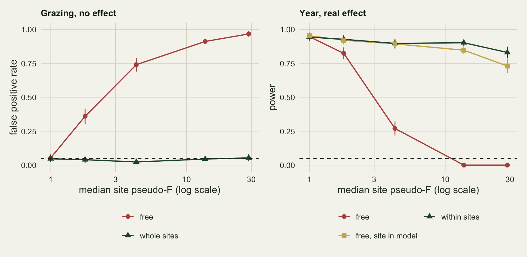
With no spread among sites (median site pseudo-F 1.00) the samples really are exchangeable and free permutation is fine: grazing is rejected in 0.053 of null data sets and the year effect is found in 0.947, against 0.943 within sites. A site standard deviation of 0.2, a median site pseudo-F of 1.79, already moves the free test of grazing to 0.360 and the free test of year to a power of 0.823; at 0.4 (site pseudo-F 4.27) they are 0.740 and 0.270. Whole-site shuffling stays between 0.023 and 0.053 across the range, and within-site shuffling keeps a power between 0.830 and 0.943; its size stays between 0.027 and 0.048. Both design-based schemes are exact under this generating model, because sites are exchangeable with each other and the samples of a site with each other, so their departures from 0.05 are Monte Carlo noise: the largest is 2.1 standard errors. The site pseudo-F is printed by adonis2(D ~ site) on the data in hand, and a value clearly above one is the warning that free permutation will mislead in both directions.
What to report
Name the permutation scheme for each term, not once for the analysis, and give the how() call or its equivalent in words: sites exchanged as whole units for the site-level treatment, samples shuffled within sites for year or for before and after, and the number of permutations. A methods sentence might read: grazing was tested by permuting whole sites (10 sites, 999 permutations) and year by permuting samples within sites (999 permutations), with Bray-Curtis dissimilarity.
ss_treat_field <- ss_perm(G_field, fm40$treat$QA, id1)
ss_site_field  <- ss_perm(G_field, fm40$site$QA, id1)
df_site_in_treat <- fm40$site$df1 - fm40$treat$df1
f_stratum <- (ss_treat_field / fm40$treat$df1) / ((ss_site_field - ss_treat_field) / df_site_in_treat)
ss_treat_w <- ss_perm(G_field, fm40$treat$QA, ps_demo$whole)
ss_site_w  <- ss_perm(G_field, fm40$site$QA, ps_demo$whole)
f_stratum_w <- (ss_treat_w / fm40$treat$df1) / ((ss_site_w - ss_treat_w) / df_site_in_treat)
p_whole_pooled  <- (1 + sum(f_perm(G_field, fm40$treat, ps_demo$whole) >= f_check["base_r", "treat"] - 1e-9)) / (1 + nrow(ps_demo$whole))
p_whole_stratum <- (1 + sum(f_stratum_w >= f_stratum - 1e-9)) / (1 + nrow(ps_demo$whole))
n_label <- choose(10, 5)
p_floor <- 2 / n_label
n_orders <- numPerms(40, ctrl_whole)
c(F_pooled = f_check["adonis2", "treat"], F_stratum = f_stratum, df_resid = fm40$treat$df2,
  df_stratum = df_site_in_treat, p_pooled = p_whole_pooled, p_stratum = p_whole_stratum)
F_pooled F_stratum df_resid df_stratum p_pooled p_stratum
4.615726 1.205748 38.000000 8.000000 0.214000 0.214000 c(labellings = n_label, p_floor = p_floor, site_orderings = n_orders) labellings p_floor site_orderings
2.520000e+02 7.936508e-03 3.628800e+06 Report the number of sites as the replication for the site-level treatment. At ten sites the whole-site test had a power of 0.587 for the grazing shift simulated here; that is the power of a comparison of five sites with five. Five grazed against five ungrazed sites allow only 252 labellings, and a labelling and its mirror image give the same sum of squares, so the exact whole-site p-value cannot fall below two in 252, about 0.008, and drawing more permutations does not lower that floor; numPerms() counts the 3,628,800 orderings of the sites instead.
The pseudo-F that adonis2() prints for grazing under whole-site shuffling divides by the pooled residual on 38 degrees of freedom; on the field data set it is 4.62. The p-value is still right, because moving whole sites leaves the site sum of squares unchanged, so that denominator and the between-site one order the permutations the same way: over the 999 base R whole-site permutations drawn earlier, both give p = 0.214. The F and its degrees of freedom, though, are those of forty samples. Report the p-value with the number of sites, or give the between-site ratio, grazing mean square over the mean square of sites within grazing, on 1 and 8 degrees of freedom: 1.21 here.
A p-value of exactly 1 can mean the scheme could not move the label. Check with diff(range(permustats(fit)$permutations)), which is zero to rounding when every permuted pseudo-F equals the observed one; then do not report the p-value, fix the scheme. A p of 1 from a spread-out null is the other failure shown here, free permutation of a within-site term, and is no more a result. The restriction also carries over to a pairwise follow-up in the manner of the pairwise PERMANOVA post: each pair’s test needs it applied to the subset of samples in that pair.
Report the site pseudo-F, adonis2(D ~ site), alongside. It tells a reader how far apart the two strata are and therefore how much a free permutation would have misled, and it costs one line.
The interaction of grazing with year varies within sites, so its permutations have to stay within sites, and grazing itself comes from a separate whole-site test. With a year effect present, shuffling raw samples within sites tests the interaction only approximately; Anderson and ter Braak 2003 discuss permuting residuals for interaction terms, and the interaction was not simulated here.
Honest limits
The design is balanced: every site has the same number of samples, in the same years. Whole-site shuffling in permute requires that (it stops with “Design must be balanced if permuting ‘strata’”), and the exact centring argument uses it. A site with a missing year breaks both; the options then are to drop to complete sites, or to test the site-level treatment on one summary per site, which is a different analysis whose behaviour was not measured here. The within-site test of year still runs when a site misses a year, since samples still move only inside their own site, but year is then no longer orthogonal to site, so fit D ~ site + year rather than D ~ year, whose year sum of squares would pick up site differences; that case was not measured here either.
The simulated sites differ by a normal shift per species on the log scale, the same size for every site, and the years by a steady trend in a few species. Real repeated surveys carry other structure that no permutation scheme here addresses: the change over time can differ between sites, samples close in time can be more alike than samples far apart, and site dispersion can differ between grazed and ungrazed sites, which a PERMANOVA reads as a location effect (Mistake 1 of the neighbour post). The within-site scheme treats the four years of a site as exchangeable, which a serial correlation would violate.
Each test used 199 permutations, enough for a five per cent test but coarse for a single p-value; a published analysis should use 999 or more. The rates carry Monte Carlo standard errors of about 0.007 near the nominal level with 1000 data sets and more for the 300-data-set cells of the sweep, so differences of a couple of hundredths between the design-based schemes are noise. The free permutation errors are many standard errors away from the level and not in doubt.
The within-site power fell at the largest site spread, to 0.830. With an additive site effect and Euclidean distance the within-site test would not see site variation at all, since the site differences cancel in every comparison inside a site. Here the site effect multiplies abundances and the distance is Bray-Curtis, so a site rich in individuals has different distances between its own years than a poor one; that was not separated here.
References
Anderson MJ 2001 Austral Ecology 26(1):32-46 (10.1111/j.1442-9993.2001.01070.pp.x)
McArdle BH, Anderson MJ 2001 Ecology 82(1):290-297 (10.1890/0012-9658(2001)082[0290:FMMTCD]2.0.CO;2)
Anderson MJ, Legendre P 1999 Journal of Statistical Computation and Simulation 62(3):271-303 (10.1080/00949659908811936)
Anderson MJ, ter Braak CJF 2003 Journal of Statistical Computation and Simulation 73(2):85-113 (10.1080/00949650215733)