library(ggplot2)
library(patchwork)

te_paper  <- "#f5f4ee"
te_ink    <- "#16241d"
te_body   <- "#2c3a31"
te_forest <- "#275139"
te_rust   <- "#b5534e"
te_gold   <- "#c9b458"
te_line   <- "#dad9ca"
te_sage   <- "#93a87f"

theme_datasheet <- function() {
  theme_minimal(base_size = 12) +
    theme(plot.background  = element_rect(fill = te_paper, colour = NA),
          panel.background = element_rect(fill = te_paper, colour = NA),
          panel.grid.major = element_line(colour = te_line, linewidth = 0.3),
          panel.grid.minor = element_blank(),
          text             = element_text(colour = te_body),
          plot.title       = element_text(colour = te_ink, face = "bold"),
          plot.subtitle    = element_text(colour = te_body),
          axis.text        = element_text(colour = te_body))
}Permutation tests with a covariate in the model
R
permutation tests
hypothesis testing
regression
collinearity
simulation
ecology tutorial
With a covariate in the model, shuffling labels or the response gives opposite wrong answers for a raw slope. Measuring in R why a t statistic repairs both.
Forty grassland plots on one hillside, each with a count of sheep dung as the measure of grazing pressure, an elevation, and a standardised score of forb richness as the response. The flock spends more of its time on the upper slopes where the sward opens out, so grazing and elevation are correlated, and elevation drives forb richness on its own. The question is whether grazing does anything once elevation is in the model, which is a test of one partial regression coefficient. Many ecologists answer it with a permutation test written by hand, and the hand-written version has to decide what to shuffle.
This site has two posts that stand on either side of that decision. Permutation tests from scratch opens its honest limits by saying that in real designs “the choice of what may be exchanged with what is a larger source of error than anything measured above”, and its repair for unequal groups is to studentise the statistic. Checking a trait environment analysis builds two permutation nulls for one statistic on one data set, plots them together, and reports that the ratio of their widths “is the entire disagreement”. A covariate in a linear model is the smallest real design there is, and there the statistic is what rescues the shuffle. The figure in the third section below is that two-curve figure with a third curve added. Multiple matrix regression with MMRR names the residual scheme used here as the published fix for its own drifting test. In an ordinary regression the t-based response shuffle that MMRR uses does not drift (see below), so the drift there does not come from the shuffle and the statistic alone; this post does not settle what it does come from.
None of this is new. Freedman and Lane 1983 proposed permuting the residuals of the model without the tested term, and Anderson and Legendre 1999 compared that scheme with shuffling the raw data and with the alternatives by simulation, in a paper whose subject is exactly the test of a partial regression coefficient in a linear model. Winkler and colleagues 2014 set the same schemes out for the general linear model. This post is a demonstration of that literature for readers who still write the loop by hand, and most of what it shows is arithmetic: the two ways the naive shuffles go wrong are closed-form variance factors, printed below before any simulation is run. The factor 1/(1 - rho^2) that drives one of them is the variance inflation factor already derived in Collinearity and VIF in ecological regression.
Forty plots, one covariate, three shuffles
Elevation is drawn from a right-skewed gamma distribution and standardised, grazing is elevation times a correlation rho plus independent noise, and forb richness is a grazing effect b_x plus 1.5 times elevation plus unit normal error. Everything is centred, so the intercept drops out of every fit.
n_plot <- 40L; b_z <- 1.5; sigma_e <- 1
n_perm <- 399L; alpha_lev <- 0.05
n_sets <- 400L; n_block <- 5L          # 400 data sets per seed block, five blocks per cell

gen_plots <- function(rho, b_x = 0, tail = "gamma") {
  elev <- if (tail == "gamma") rgamma(n_plot, 2, 1) else exp(rnorm(n_plot))
  elev <- (elev - mean(elev)) / sd(elev)
  graze <- rho * elev + sqrt(1 - rho^2) * rnorm(n_plot)
  forb <- b_x * graze + b_z * elev + rnorm(n_plot, 0, sigma_e)
  list(x = graze - mean(graze), z = elev, y = forb - mean(forb))
}

# partial slope of x given z, and its t, for every column of xm against every column of ym
part_fit <- function(xm, ym, z) {
  szz <- sum(z^2)
  ex <- xm - outer(z, colSums(z * xm) / szz)
  ry <- ym - outer(z, colSums(z * ym) / szz)
  if (ncol(ex) == 1) ex <- as.vector(ex)
  if (ncol(ry) == 1) ry <- as.vector(ry)
  sxx <- colSums(as.matrix(ex)^2)
  b <- colSums(as.matrix(ex * ry)) / sxx
  rss <- colSums(as.matrix(ry)^2) - b^2 * sxx
  list(b = b, t = b / sqrt(rss / (n_plot - 3) / sxx))
}

three_refs <- function(d, idx) {
  x <- d$x; z <- d$z; y <- d$y
  fit_z <- z * sum(z * y) / sum(z^2); res_z <- y - fit_z
  list(obs = part_fit(matrix(x), matrix(y), z),
       label = part_fit(matrix(x[idx], n_plot), matrix(y), z),        # shuffle grazing
       response = part_fit(matrix(x), matrix(y[idx], n_plot), z),     # shuffle forb richness
       fl = part_fit(matrix(x), fit_z + matrix(res_z[idx], n_plot), z)) # Freedman-Lane
}

set.seed(2809)
check <- gen_plots(0.7)
lm_row <- summary(lm(y ~ x + z, data = as.data.frame(check)))$coefficients["x", ]
own <- part_fit(matrix(check$x), matrix(check$y), check$z)
fit_gap <- max(abs(c(own$b - lm_row[1], own$t - lm_row[3])))
The three shuffles all keep the observed slope and change only the reference it is judged against. The first shuffles the grazing values among plots and refits, which is the natural extension of the two-group test. The second shuffles forb richness among plots and refits, which Anderson and Legendre call permutation of the raw data. The third fits forb richness on elevation alone, shuffles the residuals of that fit, adds them back to the fitted values and refits the full model: Freedman and Lane’s scheme. Each is run with two statistics, the raw partial slope and its t value, and the ordinary t test from lm is the seventh arm. On a check data set the hand-rolled fit and lm give the same slope and the same t value, to within floating-point rounding.
Both distortions are written down before the simulation
The observed slope has a standard error of sigma divided by the square root of the sum of squares of grazing after elevation has been regressed out, and that sum is shrunk by the factor 1 - rho^2. A shuffled grazing column is unrelated to elevation, so its sum of squares is not shrunk, and the label shuffle’s reference comes out narrower than the true sampling distribution by the square root of 1 - rho^2. A shuffled response is unrelated to both predictors, so the refit’s residual variance is the whole variance of the response rather than sigma squared, and the response shuffle’s reference comes out wider by the square root of var(y) / sigma^2. Freedman and Lane shuffle only what is left after elevation, so under the null their reference has the right width, up to a finite-sample factor of the square root of (n - 2)/(n - 1): the residuals they shuffle have lost two degrees of freedom to the intercept and elevation, and a permutation spreads them as if they had lost one. If the reference is roughly normal, a factor k on its width turns a nominal two-sided five per cent test into one that rejects at 2 Phi(-1.96 k).
q_nom <- qnorm(1 - alpha_lev / 2)
rho_hi <- 0.7
w_label <- function(rho, b_x = 0) sqrt(1 - rho^2) * sqrt(1 + b_x^2 * (1 - rho^2) / sigma_e^2)
w_resp  <- function(rho, b_x = 0) sqrt((b_x^2 + b_z^2 + 2 * b_x * b_z * rho + sigma_e^2) / sigma_e^2)
w_fl    <- function(rho, b_x = 0) sqrt((n_plot - 2) / (n_plot - 1)) * sqrt(1 + b_x^2 * (1 - rho^2) / sigma_e^2)
lev_pred <- function(k) 2 * pnorm(-q_nom * k)
k_lab <- w_label(rho_hi); k_resp <- w_resp(rho_hi)
pred_lab <- lev_pred(k_lab); pred_resp <- lev_pred(k_resp)
pred_lab_t <- 2 * pt(-q_nom * k_lab, n_plot - 3)   # the same factor read against t(37)
c(label_factor = k_lab, label_level = pred_lab,
  response_factor = k_resp, response_level = pred_resp)
label_factor label_level response_factor response_level
0.7141428429 0.1616048959 1.8027756377 0.0004102896 At a grazing to elevation correlation of 0.7 the label shuffle’s reference is 0.714 times the right width and should reject a true null at about 0.162. The response shuffle’s reference is 1.803 times the right width, whatever the correlation, because the factor depends only on how much elevation explains; it should reject at about 0.0004. Those two numbers are the predictions the simulation has to land on. The functions also carry a grazing effect b_x, which matters later: a real effect adds its own variance to what gets shuffled.
Three references for one slope
One null data set at a correlation of 0.7, the first one the seed gives, with 3999 permutations for each shuffle so that the shapes are smooth.
set.seed(4417)
one_d <- gen_plots(rho_hi)
idx_big <- replicate(3999, sample.int(n_plot))
refs <- three_refs(one_d, idx_big)
p_one <- function(ref, o) (1 + sum(abs(ref) >= abs(o))) / (length(ref) + 1)
one_tab <- sapply(c("label", "response", "fl"), function(s)
  c(p_raw = p_one(refs[[s]]$b, refs$obs$b), p_t = p_one(refs[[s]]$t, refs$obs$t),
    sd_raw = sd(refs[[s]]$b)))
one_se <- refs$obs$b / refs$obs$t
one_p_ols <- 2 * pt(-abs(refs$obs$t), n_plot - 3)
one_spread <- max(one_tab["p_raw", ]) / min(one_tab["p_raw", ])
one_r <- cor(one_d$x, one_d$z)
one_k_r <- sqrt(1 - one_r^2)                     # label factor at this draw's own correlation
one_k_full <- one_k_r * sqrt((n_plot - 3 + refs$obs$t^2) / (n_plot - 1)) * (n_plot - 1) / (n_plot - 2)
round(one_tab, 4)
label response fl
p_raw 0.0522 0.3862 0.0978
p_t 0.1108 0.1128 0.1040
sd_raw 0.1292 0.2857 0.1511On this data set the observed grazing slope is 0.248 with a standard error of 0.150, and the ordinary t test gives a p value of 0.107. Compared as a raw slope, the label shuffle gives 0.0522, the response shuffle 0.3862 and Freedman-Lane 0.0978. The spreads of the three references are 0.859, 1.899 and 1.005 times the standard error. Compared as t values, the three p values are 0.1108, 0.1128 and 0.1040.
ref_lev <- c("shuffle grazing", "shuffle forb richness", "Freedman-Lane")
ref_col <- c(te_rust, te_gold, te_forest); names(ref_col) <- ref_lev
dens_of <- function(stat) do.call(rbind, lapply(seq_along(ref_lev), function(j) {
  v <- refs[[c("label", "response", "fl")[j]]][[stat]]
  data.frame(value = v, scheme = factor(ref_lev[j], levels = ref_lev))
}))
panel_ref <- function(stat, obs, xlab, ttl) {
  ggplot(dens_of(stat), aes(value, colour = scheme)) +
    geom_density(linewidth = 0.9, adjust = 1.2) +
    geom_vline(xintercept = obs, colour = te_ink, linetype = "dashed", linewidth = 0.6) +
    scale_colour_manual(values = ref_col, name = NULL) +
    labs(x = xlab, y = "density", title = ttl) +
    theme_datasheet() + theme(legend.position = "bottom")
}
(panel_ref("b", refs$obs$b, "partial slope of grazing", "Raw slope: three widths") +
  panel_ref("t", refs$obs$t, "t value of grazing", "t value: one width")) +
  plot_layout(guides = "collect") +
  plot_annotation(theme = theme_datasheet() + theme(legend.position = "bottom"))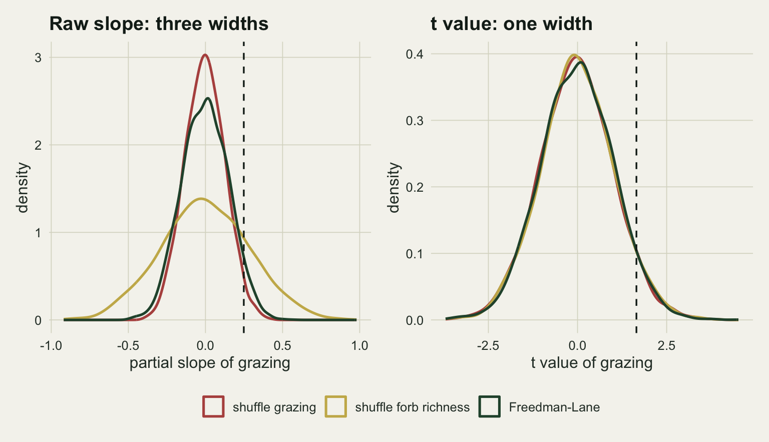
The rates land on the formulas
Three null cells: no correlation, a correlation of 0.7 with the gamma elevation, and the same correlation with a much longer-tailed covariate, a standardised lognormal, in which a few plots sit far above the rest. Each cell is five seed blocks of 400 data sets with 399 permutations each, fixed before anything was run. The width ratio for each data set is the standard deviation of the permuted raw slopes divided by the ordinary standard error on the same data set.
arm_key <- c("ols_t", "lab_b", "lab_t", "resp_b", "resp_t", "fl_b", "fl_t")
arm_lab <- c("OLS t test", "shuffle grazing, raw slope", "shuffle grazing, t",
             "shuffle response, raw slope", "shuffle response, t",
             "Freedman-Lane, raw slope", "Freedman-Lane, t")
one_set <- function(rho, b_x = 0, tail = "gamma") {
  r <- three_refs(gen_plots(rho, b_x, tail), replicate(n_perm, sample.int(n_plot)))
  pv <- function(ref, o) (1 + sum(abs(ref) >= abs(o))) / (n_perm + 1)
  se <- r$obs$b / r$obs$t
  c(ols_t = 2 * pt(-abs(r$obs$t), n_plot - 3),
    lab_b = pv(r$label$b, r$obs$b), lab_t = pv(r$label$t, r$obs$t),
    resp_b = pv(r$response$b, r$obs$b), resp_t = pv(r$response$t, r$obs$t),
    fl_b = pv(r$fl$b, r$obs$b), fl_t = pv(r$fl$t, r$obs$t),
    w_lab = sd(r$label$b) / se, w_resp = sd(r$response$b) / se, w_fl = sd(r$fl$b) / se)
}
run_cell <- function(rho, b_x, tail, seed0) {
  blocks <- lapply(seq_len(n_block), function(k) {
    set.seed(seed0 + k)
    vapply(seq_len(n_sets), function(i) one_set(rho, b_x, tail), numeric(10))
  })
  rej <- t(vapply(blocks, function(m) rowMeans(m[arm_key, ] <= alpha_lev), numeric(7)))
  allm <- do.call(cbind, blocks)
  list(rej = rej, n_rej = rowSums(allm[arm_key, ] <= alpha_lev),
       width = apply(allm[c("w_lab", "w_resp", "w_fl"), ], 1, median))
}
cell_null0 <- run_cell(0, 0, "gamma", 61000)
cell_null7 <- run_cell(rho_hi, 0, "gamma", 62000)
cell_tail7 <- run_cell(rho_hi, 0, "lnorm", 63000)
n_cell <- n_sets * n_block
mcse_nom <- sqrt(alpha_lev * (1 - alpha_lev) / n_cell)
lab_pool <- unname(cell_null7$n_rej["lab_b"]) / n_cell
lab_pool_se <- sqrt(lab_pool * (1 - lab_pool) / n_cell)
med <- function(cell, key) median(cell$rej[, key])
rng <- function(cell, key) sprintf("%.3f [%.3f, %.3f]", median(cell$rej[, key]),
                                   min(cell$rej[, key]), max(cell$rej[, key]))
w_err <- c(abs(cell_null7$width["w_lab"] / k_lab - 1), abs(cell_null7$width["w_resp"] / k_resp - 1),
           abs(cell_null7$width["w_fl"] / w_fl(rho_hi) - 1))
The measured width ratios at a correlation of 0.7 are 0.716 for the label shuffle against the formula’s 0.714, 1.795 for the response shuffle against 1.803, and 0.986 for Freedman-Lane against 0.987, the finite-sample factor itself. The largest relative miss is 0.4 per cent. The simulation is confirming arithmetic, not finding anything.
Rejection rates of a true null, as median [lowest block, highest block] over five blocks, with a Monte Carlo standard error of 0.0049 for a pooled rate of five per cent over 2000 data sets. At a correlation of 0.7, shuffling grazing and comparing raw slopes rejects at 0.172 [0.138, 0.193], or 0.1655 pooled over all 2000 data sets with a Monte Carlo standard error of 0.0083, against the formula’s 0.162. Reading the observed t value against a t distribution on 37 degrees of freedom instead of the normal puts the prediction at 0.170. The two predictions sit 0.47 and 0.53 Monte Carlo standard errors from the pooled rate, so the simulation cannot tell them apart. Shuffling the response and comparing raw slopes rejects in 1 of 2000 data sets, where the formula’s 0.0004 predicts about 0.8. Neither number is a finding: both are the closed forms above.
The formulas predict the repair in large samples; whether it holds at forty plots with a skewed covariate is what the simulation measures. Divide each permuted slope by its own standard error and the label shuffle rejects at 0.048 [0.037, 0.065], the response shuffle at 0.052 [0.043, 0.065]. Freedman-Lane rejects at 0.048 [0.035, 0.065] on the raw slope and 0.045 [0.035, 0.065] on the t value, and the ordinary t test at 0.050 [0.037, 0.062]. The studentised statistic works because each permuted t is divided by a standard error computed from the permuted fit, which carries the same factor that distorted the raw slope: the label shuffle’s standard error is not shrunk by collinearity either, and the response shuffle’s residual variance is inflated by elevation’s share too.
With no correlation the label shuffle’s factor is one, and its raw slope rejects at 0.058 [0.048, 0.058]. The response shuffle’s factor does not depend on the correlation at all, and its raw slope rejects in 0 of 2000 data sets, against the same prediction of about 0.8. Its studentised version is at 0.052 [0.045, 0.060]. With the long-tailed covariate at a correlation of 0.7, the widths are 0.712, 1.810 and 0.984, and the repaired arms reject at 0.048 [0.028, 0.055] for the studentised label shuffle, 0.048 [0.025, 0.055] for the studentised response shuffle and 0.045 [0.028, 0.060] for Freedman-Lane on t.
A real effect widens the response shuffle again
The response shuffle’s factor has var(y) in it, and var(y) contains the grazing effect the test is looking for. So when grazing does act on forbs, the reference that was already too wide grows with the effect. That is still arithmetic, the same formula with b_x switched on, but it has a consequence the null factor hides: the loss of power is much larger than a fixed inflation would predict. The runs below add grazing effects of 0.4, 0.8 and 1.2 at a correlation of 0.7, with the same block structure.
bx_grid <- c(0.4, 0.8, 1.2)
cell_alt <- lapply(seq_along(bx_grid), function(j) run_cell(rho_hi, bx_grid[j], "gamma", 64000 + 100 * j))
names(cell_alt) <- sprintf("%.1f", bx_grid)
alt8 <- cell_alt[["0.8"]]
se_pop <- function(rho) sigma_e / sqrt((n_plot - 2) * (1 - rho^2))
pow_pred <- function(k, b_x, rho = rho_hi) {
  delta <- b_x / se_pop(rho)
  pnorm(delta - q_nom * k) + pnorm(-delta - q_nom * k)
}
k_resp_alt8 <- w_resp(rho_hi, 0.8)
pred_fixed8 <- pow_pred(k_resp, 0.8); pred_grow8 <- pow_pred(k_resp_alt8, 0.8)
pred_ols8 <- pow_pred(1, 0.8)
width_rise <- alt8$width["w_resp"] / cell_null7$width["w_resp"] - 1
mcse_pow <- sqrt(0.25 / n_cell)
fl_crit <- sqrt(q_nom^2 * (n_plot - 3) / (n_plot - 1 - q_nom^2))   # Freedman-Lane raw slope as a t cutoff
At a grazing effect of 0.8 the response shuffle’s measured width ratio is 2.366, against 1.795 under the null: 32 per cent wider, and the formula with the effect switched on gives 2.360. The label shuffle’s ratio has moved to 0.821 (formula 0.822) and Freedman-Lane’s to 1.127 (formula 1.137), because a real grazing effect is also part of what Freedman-Lane shuffles. Its t statistic absorbs that in the same way, and its raw slope loses nothing either (power 0.917 against the t test’s 0.917, below): the extra width in its reference is made of the observed slope itself, so the raw-slope test is roughly a t test with a cutoff of 2.011 instead of 2.026.
Power at that effect, as median [lowest, highest block], with a Monte Carlo standard error of at most 0.011 for a pooled rate: the ordinary t test 0.917 [0.890, 0.927], the studentised label shuffle 0.915 [0.895, 0.925], the studentised response shuffle 0.910 [0.885, 0.920], Freedman-Lane 0.917 [0.892, 0.930] on the raw slope and 0.917 [0.877, 0.925] on t. The raw response shuffle detects the effect at 0.155 [0.147, 0.198]. A normal approximation with the null factor held fixed would predict 0.495 for it; with the factor that grows with the effect it predicts 0.135, and the same approximation gives 0.941 for the ordinary t test. The raw label shuffle detects the effect at 0.968 [0.953, 0.973], which is not power: that arm rejects 0.172 of true nulls too.
bx_all <- c(0, bx_grid)
cells_all <- c(list(cell_null7), cell_alt)
w_meas <- do.call(rbind, lapply(seq_along(bx_all), function(j)
  data.frame(b_x = bx_all[j], scheme = factor(ref_lev, levels = ref_lev),
             width = unname(cells_all[[j]]$width))))
bx_fine <- seq(0, 1.2, length.out = 61)
w_line <- rbind(data.frame(b_x = bx_fine, scheme = ref_lev[1], width = w_label(rho_hi, bx_fine)),
                data.frame(b_x = bx_fine, scheme = ref_lev[2], width = w_resp(rho_hi, bx_fine)),
                data.frame(b_x = bx_fine, scheme = ref_lev[3], width = w_fl(rho_hi, bx_fine)))
w_line$scheme <- factor(w_line$scheme, levels = ref_lev)
p_w <- ggplot(w_line, aes(b_x, width, colour = scheme)) +
  geom_hline(yintercept = 1, colour = te_body, linetype = "dashed", linewidth = 0.4) +
  geom_line(linewidth = 0.9) +
  geom_point(data = w_meas, size = 2.4) +
  scale_colour_manual(values = ref_col, name = NULL) +
  guides(colour = guide_legend(ncol = 1)) +
  labs(x = "grazing effect", y = "reference sd / true standard error",
       title = "Reference width", subtitle = "lines: closed form; points: simulation") +
  theme_datasheet() + theme(legend.position = "bottom")
pow_meas <- do.call(rbind, lapply(seq_along(bx_all), function(j)
  data.frame(b_x = bx_all[j],
             arm = factor(c("shuffle response, raw slope", "Freedman-Lane, t", "shuffle response, t"),
                          levels = c("shuffle response, raw slope", "Freedman-Lane, t", "shuffle response, t")),
             power = colMeans(cells_all[[j]]$rej[, c("resp_b", "fl_t", "resp_t")]))))
pow_line <- rbind(data.frame(b_x = bx_fine, pred = "null width held fixed",
                             power = pow_pred(k_resp, bx_fine)),
                  data.frame(b_x = bx_fine, pred = "width grows with the effect",
                             power = pow_pred(w_resp(rho_hi, bx_fine), bx_fine)))
p_p <- ggplot() +
  geom_line(data = pow_line, aes(b_x, power, linetype = pred), colour = te_gold, linewidth = 0.8) +
  geom_point(data = pow_meas, aes(b_x, power, shape = arm, colour = arm), size = 2.4) +
  scale_colour_manual(values = c(te_gold, te_forest, te_ink), name = NULL) +
  scale_shape_manual(values = c(16, 17, 1), name = NULL) +
  scale_linetype_manual(values = c("dotted", "solid"), name = NULL) +
  scale_y_continuous(limits = c(0, 1)) +
  guides(colour = guide_legend(ncol = 1), shape = guide_legend(ncol = 1),
         linetype = guide_legend(ncol = 1)) +
  labs(x = "grazing effect", y = "rejection rate", title = "Power",
       subtitle = "gold lines: predicted, raw response shuffle") +
  theme_datasheet() + theme(legend.position = "bottom", legend.box = "vertical")
p_w + p_p + plot_annotation(theme = theme_datasheet())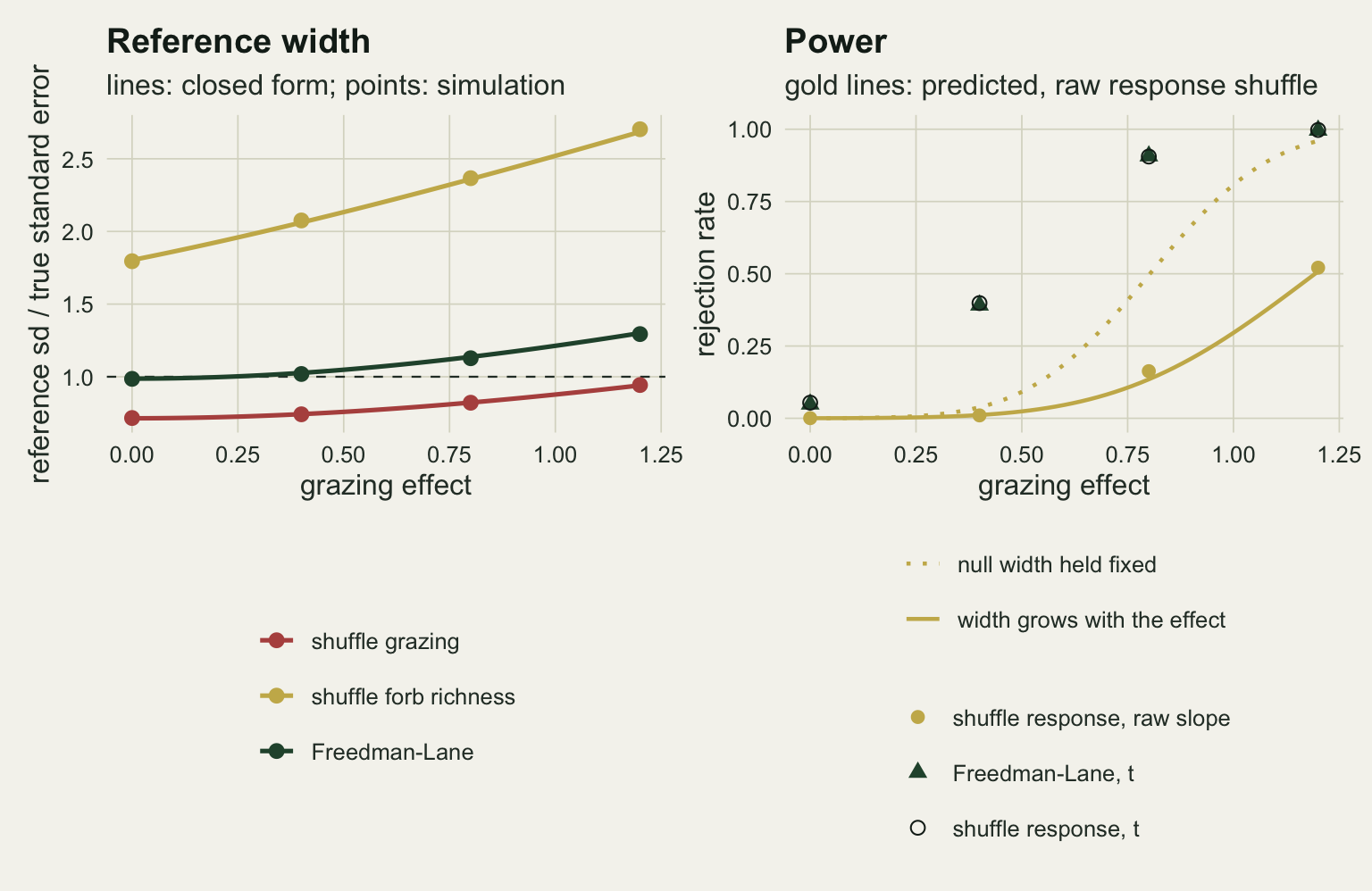
cell_lev <- c("rho 0", "rho 0.7", "rho 0.7, long tail")
rate_long <- function(cell, lab) data.frame(
  arm = factor(arm_lab, levels = rev(arm_lab)), cell = factor(lab, levels = cell_lev),
  med = apply(cell$rej, 2, median), lo = apply(cell$rej, 2, min), hi = apply(cell$rej, 2, max))
null_tab <- rbind(rate_long(cell_null0, cell_lev[1]), rate_long(cell_null7, cell_lev[2]),
                  rate_long(cell_tail7, cell_lev[3]))
cell_col <- c(te_sage, te_ink, te_ink); names(cell_col) <- cell_lev
cell_shp <- c(16, 16, 2); names(cell_shp) <- cell_lev
p_null <- ggplot(null_tab, aes(med, arm, colour = cell, shape = cell)) +
  geom_vline(xintercept = alpha_lev, colour = te_body, linetype = "dashed", linewidth = 0.4) +
  geom_errorbar(aes(xmin = lo, xmax = hi), orientation = "y", width = 0, linewidth = 0.5,
                position = position_dodge(width = 0.6)) +
  geom_point(size = 2.1, position = position_dodge(width = 0.6)) +
  scale_colour_manual(values = cell_col, name = NULL) +
  scale_shape_manual(values = cell_shp, name = NULL) +
  labs(x = "rejection rate, true null", y = NULL, title = "Level") +
  theme_datasheet() + theme(legend.position = "bottom")
pow_tab <- rate_long(alt8, cell_lev[2])
p_pow <- ggplot(pow_tab, aes(med, arm)) +
  geom_errorbar(aes(xmin = lo, xmax = hi), orientation = "y", width = 0, linewidth = 0.5,
                colour = te_ink) +
  geom_point(size = 2.3, colour = te_ink) +
  scale_x_continuous(limits = c(0, 1)) +
  labs(x = "rejection rate, grazing effect 0.8", y = NULL, title = "Power, rho 0.7") +
  theme_datasheet() + theme(axis.text.y = element_blank())
p_null + p_pow + plot_layout(widths = c(1.4, 1)) + plot_annotation(theme = theme_datasheet())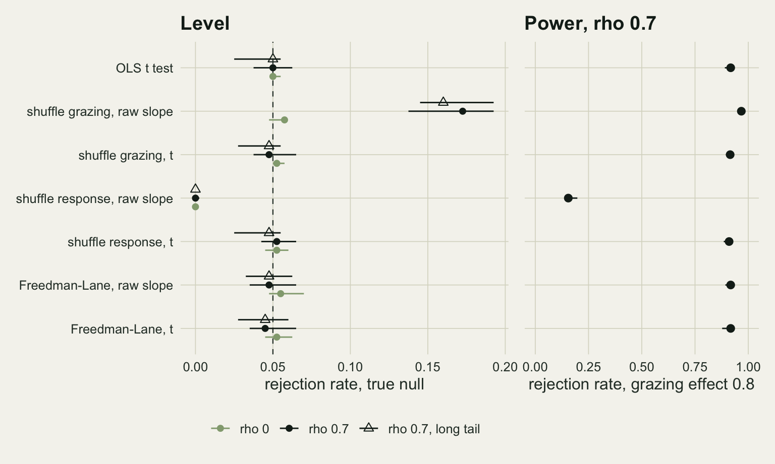
What to report
With any covariate in the model, compare t values (or F values) under the shuffle, not raw coefficients. The coefficient can still be the number the paper reports and interprets; it should not be the statistic the permutation p value is computed from. Every studentised arm here held its level and matched the ordinary t test’s power, whichever of the three shuffles it rode on.
If the analysis has to permute a raw coefficient, for instance because a custom statistic has no standard error, use Freedman and Lane’s scheme: fit the model without the tested term, shuffle its residuals, add them back to its fitted values, refit. Here it held its level on the raw slope as well as on t. Anderson and Legendre 1999 found the reduced-model scheme the most consistently reliable of the schemes they compared, and found raw-data permutation unstable when the covariate held an extreme outlier.
Say which shuffle and which statistic were used, and the number of permutations, next to the p value. “A permutation test” does not identify a procedure once a covariate is present: the single data set in the figure above gives raw-slope p values that differ by a factor of 7.4 across the three shuffles, and a different draw can put them on opposite sides of 0.05.
For readers of vegan output: in version 2.6-4, checked for this post by feeding it the same permutation matrix as the code here, adonis2 with by = "terms" (grazing entered after elevation) or by = "margin" reproduces the studentised response shuffle’s p value exactly, since its pseudo-F is a ratio statistic and it permutes the raw rows; anova on an rda with Condition(elevation) and the default reduced model reproduces the studentised Freedman-Lane p value. With by = "terms" and grazing entered first, grazing is tested without adjusting for elevation, which is a different hypothesis. Newer versions change three things. From vegan 2.6-8 the default is by = NULL, an omnibus test of the whole model, so pass by = "margin" explicitly. From 2.7-2, according to its NEWS file, anova on a partial rda residualises the constraints, which changes results for models with a Condition term, so the rda match above holds for 2.6-4 and was not rechecked on later versions. The NEWS file for 2.8-0 adds Condition() to the adonis2 formula; whether that then permutes like the rda version was not checked here.
Honest limits
Everything here is one covariate, one tested term, forty plots and normal errors. Both width formulas are large-sample statements and assume a roughly normal reference. The simulation adds nothing to them; its contribution is to show that the studentised versions and Freedman-Lane held their level at this sample size with a skewed covariate and with a longer-tailed one, and that the raw response shuffle’s power loss follows the widening formula rather than the null one.
The long-tailed covariate is a standardised lognormal, which puts a few plots far out but is not the single extreme outlier Anderson and Legendre found to destabilise raw-data permutation. That case was not run, and neither were non-normal errors, where they found the permutation schemes more powerful than the ordinary t test. Here, with normal errors, the ordinary t test is exact and every repaired arm only matches it.
Two schemes in the literature were not measured. ter Braak’s scheme permutes the residuals of the full model; Anderson and ter Braak 2003 compare it with Freedman-Lane for factorial designs. Kennedy’s scheme, which Anderson and Legendre found inflates the type I error, residualises both grazing and forb richness on elevation before shuffling. Readers using either should not take the rates above as theirs.
The power predictions in the widening figure use a normal approximation with a population standard error and the population width; they ignore the t distribution and the spread of the width from data set to data set. They are there to show which formula the measured power follows, not to replace it.
The one-data-set figure is the first draw from its seed. Its widths are one data set’s, not the medians: the label shuffle’s is 0.859 times the standard error there against the formula’s 0.714, because this draw’s sample correlation between grazing and elevation is 0.559, which puts the square root of 1 - r^2 at 0.829. The rest is the observed slope, which stays in the residual variance of every label-shuffled refit (its t value here is 1.65), plus a finite-sample term; with both included the same arithmetic gives 0.859. Another draw moves the observed value and the three widths around the formulas; the ordering of the three curves is what carries over.
References
Freedman D, Lane D 1983 Journal of Business and Economic Statistics 1(4):292-298 (10.1080/07350015.1983.10509354)
Anderson MJ, Legendre P 1999 Journal of Statistical Computation and Simulation 62(3):271-303 (10.1080/00949659908811936)
Anderson MJ, ter Braak CJF 2003 Journal of Statistical Computation and Simulation 73(2):85-113 (10.1080/00949650215733)
Winkler AM, Ridgway GR, Webster MA, Smith SM, Nichols TE 2014 NeuroImage 92:381-397 (10.1016/j.neuroimage.2014.01.060)