library(ggplot2)
library(patchwork)

te_paper  <- "#f5f4ee"
te_ink    <- "#16241d"
te_body   <- "#2c3a31"
te_forest <- "#275139"
te_rust   <- "#b5534e"
te_gold   <- "#c9b458"
te_line   <- "#dad9ca"

theme_datasheet <- function() {
  theme_minimal(base_size = 12) +
    theme(plot.background  = element_rect(fill = te_paper, colour = NA),
          panel.background = element_rect(fill = te_paper, colour = NA),
          panel.grid.major = element_line(colour = te_line, linewidth = 0.3),
          panel.grid.minor = element_blank(),
          text             = element_text(colour = te_body),
          plot.title       = element_text(colour = te_ink, face = "bold"),
          axis.text        = element_text(colour = te_body))
}

n_a <- 8; n_b <- 8
set.seed(44)
ctrl <- round(rnorm(n_a, 12, 2.2), 2)
trt  <- round(rnorm(n_b, 12 + 4.2, 2.2), 2)
pooled <- c(ctrl, trt)
gap <- function(i) abs(mean(pooled[i]) - mean(pooled[-i]))
observed <- gap(seq_len(n_a))Permutation tests from scratch
R
hypothesis testing
statistics
ecology tutorial
A permutation test is called exact, and a Monte Carlo one has a floor it cannot report below. Here is where that floor sits and what it hides in ecology.
A permutation test is the one procedure in the toolkit that seems to need no assumptions. Shuffle the group labels, recompute the statistic, count how often the shuffled version beats the one you observed. No normality, no variance assumption, no reliance on a limiting distribution, and the word attached to it in every textbook is exact.
Two things get lost between that description and the line of output. The first is that almost nobody enumerates the permutations: they draw a few hundred or a few thousand at random, which turns an exact test into an estimate of one, with an estimate’s error and a hard floor below which it cannot report. The second is that exactness holds for a null hypothesis of complete exchangeability, which is not the null hypothesis most ecologists mean when they compare two groups.
This post writes the test out by hand for a small two-sample problem, enumerates every possible split so that the exact answer is known, and then measures what the Monte Carlo version does to it. The design question of which units may be shuffled is covered elsewhere on the site; here the shuffling is unrestricted and the question is what the p value itself can and cannot say.
Sixteen plots, two treatments
Eight control plots and eight treated plots, one response per plot. The test statistic is the absolute difference in means, and the null hypothesis is that treatment did nothing at all to any plot, so the sixteen values would have come out the same whichever label each plot had been given.
The two groups differ by 3.93 units. Whether that is more than label shuffling would produce is the whole question, and with sixteen plots it can be answered without any sampling at all.
Every split, counted
There are 12870 ways to choose which eight of the sixteen plots carry the control label. That is a number combn() will produce in a fraction of a second, so the permutation distribution here is not estimated: it is the complete list.
splits   <- combn(n_a + n_b, n_a)
perm_gap <- apply(splits, 2, gap)
n_split  <- ncol(splits)

as_extreme <- sum(perm_gap >= observed - 1e-12)
p_exact    <- as_extreme / n_split
p_floor    <- 2 / n_split
attainable <- length(unique(round(sapply(sort(unique(round(perm_gap, 10))),
                                         function(v) mean(perm_gap >= v - 1e-12)), 10)))
p_t <- t.test(ctrl, trt, var.equal = TRUE)$p.value

alpha    <- 0.05
n_perm   <- 999
small_n  <- 6
small_ct <- choose(2 * small_n, small_n)
small_fl <- 2 / small_ct
big_ct   <- choose(24, 12)
se_at_a  <- sqrt(alpha * (1 - alpha) / n_perm)
Of the 12870 splits, 12 give a difference at least as large as the one observed, so the exact p value is 0.00093. The equal variance t test on the same data returns 0.00064, which is close enough to be reassuring and different enough to be worth knowing.
ggplot(data.frame(g = perm_gap), aes(g)) +
  geom_histogram(bins = 60, fill = te_forest, colour = NA) +
  geom_vline(xintercept = observed, colour = te_rust, linetype = "dashed",
             linewidth = 0.9) +
  annotate("text", x = observed, y = Inf, vjust = 1.8, hjust = 1.06,
           label = "observed", colour = te_rust, fontface = "bold", size = 3.6) +
  labs(x = "absolute difference in group means", y = "splits",
       title = "All 12870 splits, not a sample of them") +
  theme_datasheet()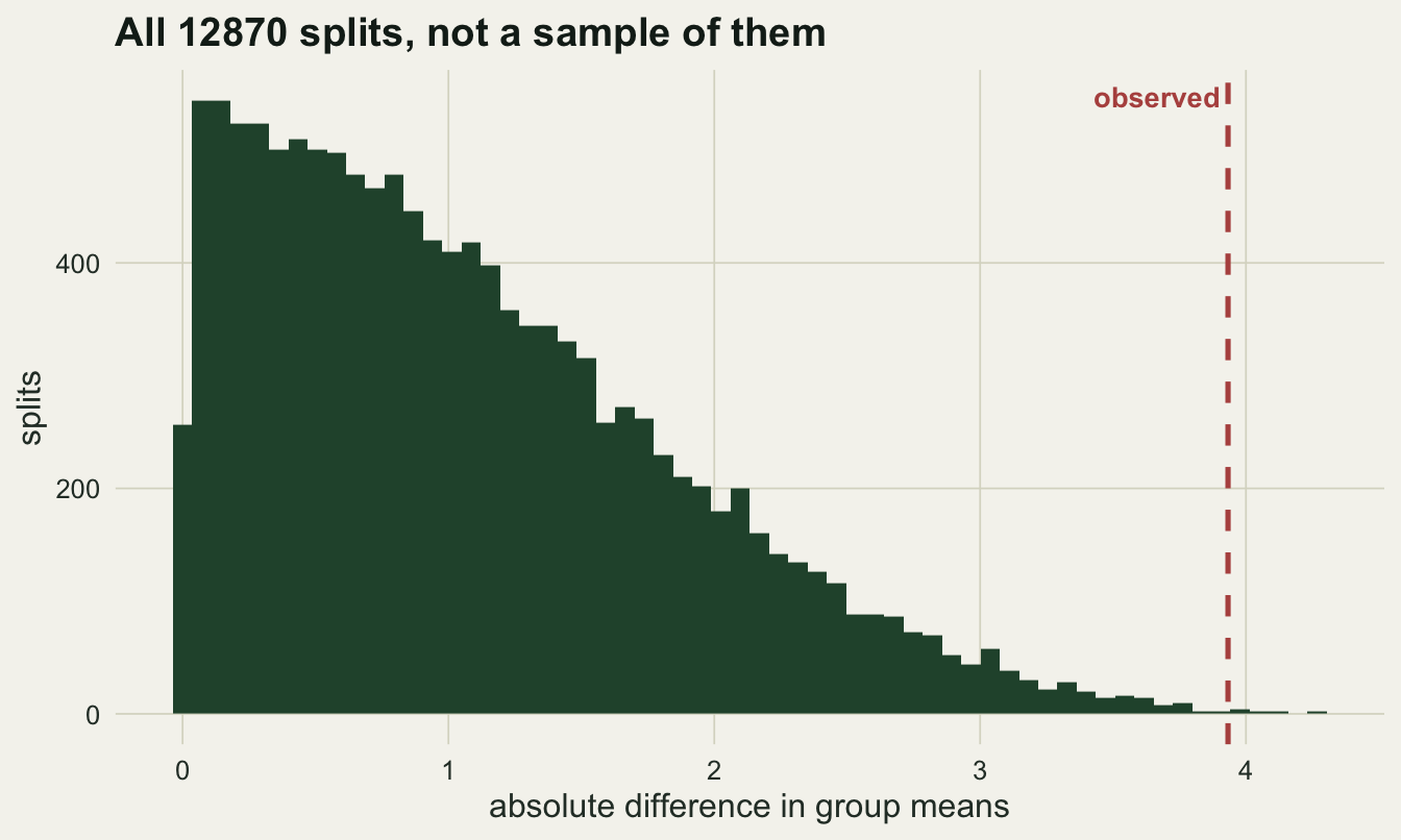
The complete enumeration also fixes the resolution of the test. The smallest p value these data can produce is 0.000155, which is two splits out of 12870: the most extreme labelling and its mirror image. Between that and one there are 1228 attainable values and nothing in between them. A permutation p value is a fraction with a fixed denominator, and for small designs the ladder is coarse. Six plots against six gives 924 splits and a smallest possible p value of 0.0022, so a six against six experiment cannot report below that figure no matter how large the effect.
What the Monte Carlo version can report
Enumeration stops being possible quickly. Twelve against twelve is already 2 704 156 splits, and any design with more than a couple of dozen units has to be sampled. The standard estimator adds the observed arrangement to the sampled ones, which is what keeps the p value from ever being zero:
grand <- sum(pooled)
mc_p <- function(B) {
  totals <- replicate(B, sum(pooled[sample(n_a + n_b, n_a)]))
  drawn  <- abs(totals / n_a - (grand - totals) / n_b)
  (1 + sum(drawn >= observed - 1e-12)) / (B + 1)
}
set.seed(6215)
n_runs  <- 300
mc_999  <- replicate(n_runs, mc_p(n_perm))
mc_9999 <- replicate(n_runs, mc_p(10 * (n_perm + 1) - 1))

floor_999   <- 1 / (n_perm + 1)
at_floor    <- 100 * mean(mc_999 <= floor_999 + 1e-12)
med_999     <- median(mc_999)
twice_exact <- 100 * mean(mc_999 >= 2 * p_exact)
b_needed    <- (1 - p_exact) / (p_exact * 0.04)
With 999 permutations the smallest reportable p value is 0.001, and the exact answer for these data is 0.00093, which is below it. Running the sampled test 300 times on the same fixed dataset, 35 per cent of runs land exactly on the floor and the median run reports 0.002. In 65 per cent of runs the reported value is at least twice the truth.
panel <- function(v, B, ttl) {
  ggplot(data.frame(p = v), aes(p)) +
    geom_histogram(bins = 24, fill = te_gold, colour = NA) +
    geom_vline(xintercept = p_exact, colour = te_forest, linewidth = 1) +
    geom_vline(xintercept = 1 / (B + 1), colour = te_rust, linetype = "dashed",
               linewidth = 0.8) +
    labs(x = "reported p value", y = "runs", title = ttl) +
    theme_datasheet()
}
(panel(mc_999, 999, "999 permutations") +
  panel(mc_9999, 9999, "9999 permutations")) + plot_annotation(theme = theme_datasheet())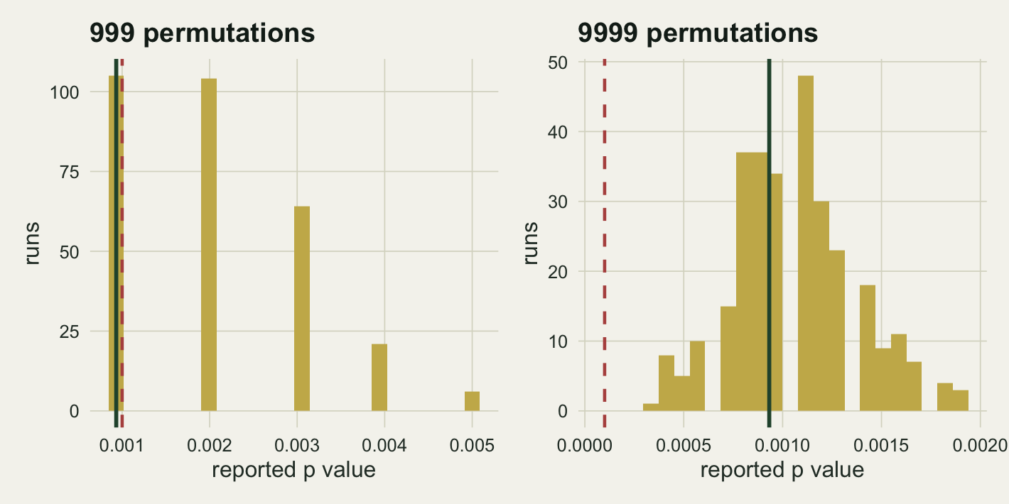
Ten thousand permutations puts the estimate on the right scale, and the spread is still wide in relative terms because a p value near 0.001 is a count of about ten events. Resolving it to within a fifth of its own size takes roughly 26800 permutations. That is not a large computation for a two-sample difference in means; it is a large computation for a PERMANOVA on a big community matrix, which is exactly where the default of 999 tends to be left alone.
None of this matters when the p value is near 0.05, where 999 permutations give a standard error of about 0.007 and the decision rarely turns on it. It matters when a small p value is being used as a quantity: reported to three decimals in a table, compared between analyses, or fed into a multiple comparison correction that treats the ordering of small p values as information. Phipson and Smyth made the same argument in 2010, and their recommendation for genomics work applies here as well: report the p value with its number of permutations attached, and never report zero.
Exact for which null
The exactness result says that if the labels are exchangeable under the null, the permutation p value has the level it claims. Exchangeable means every arrangement of the observed values was equally likely, which requires the groups to share a distribution, not merely a mean. Ecological data with a treatment that changes the variance, or with groups of unequal size, will not satisfy it.
The measurement is direct: generate data where both group means are zero, so every rejection is a false positive, and vary the group sizes and the variances.
perm_pair <- function(na, nb, sa, sb, B = 999) {
  n <- na + nb
  v <- c(rnorm(na, 0, sa), rnorm(nb, 0, sb))
  picks <- matrix(0, B, n)
  for (k in seq_len(B)) picks[k, sample(n, na)] <- 1
  picks <- rbind(c(rep(1, na), rep(0, nb)), picks)   # row one is the observed split
  s_a <- as.vector(picks %*% v); q_a <- as.vector(picks %*% (v * v))
  s_b <- sum(v) - s_a;           q_b <- sum(v * v) - q_a
  m_a <- s_a / na; m_b <- s_b / nb
  v_a <- (q_a - na * m_a^2) / (na - 1)
  v_b <- (q_b - nb * m_b^2) / (nb - 1)
  raw <- abs(m_a - m_b)
  stu <- raw / sqrt(v_a / na + v_b / nb)
  c(raw = sum(raw >= raw[1] - 1e-12) / (B + 1),
    stu = sum(stu >= stu[1] - 1e-12) / (B + 1))
}

set.seed(202)
n_rep   <- 1200
designs <- list(c(10, 10, 3, 1), c(8, 24, 1, 3), c(8, 24, 3, 1), c(6, 30, 3, 1))
err <- do.call(rbind, lapply(designs, function(cf) {
  reps <- replicate(n_rep, perm_pair(cf[1], cf[2], cf[3], cf[4]))
  data.frame(design = sprintf("n %d/%d, sd %d/%d", cf[1], cf[2], cf[3], cf[4]),
             raw = mean(reps["raw", ] <= alpha),
             studentised = mean(reps["stu", ] <= alpha))
}))
se_rate  <- sqrt(alpha * (1 - alpha) / n_rep)
same_p   <- identical(err$raw[1], err$studentised[1])
print(transform(err, raw = round(raw, 3), studentised = round(studentised, 3)),
      row.names = FALSE)
design raw studentised
n 10/10, sd 3/1 0.059 0.059
n 8/24, sd 1/3 0.003 0.044
n 8/24, sd 3/1 0.196 0.058
n 6/30, sd 3/1 0.288 0.069The first row is not a coincidence. With equal group sizes the two statistics give the same p value on every dataset, which is why the rate is identical to the last digit: they agree exactly. The reason is arithmetic. The total sum of squares does not change when the labels are shuffled, so with equal group sizes the pooled within group variance is a decreasing function of the difference in means, and dividing by it is a monotone transformation that cannot reorder the permutation distribution. Studentising can only change an answer when the groups differ in size. The rate itself, 0.059 against a nominal 0.05, is within 1.5 standard errors of the target. Once the sizes are unequal the direction of the imbalance decides everything. When the smaller group is the more variable one the test rejects a true null 19.6 per cent of the time at eight against twenty four, and 28.8 per cent at six against thirty. Reverse the variances and the same test becomes so conservative it rejects 0.3 per cent of the time, which is not safety: it is power thrown away.
Studentising the statistic repairs most of it. Divide the difference in means by its own standard error, computed separately within each shuffled group, and permute that instead. The same three designs give 5.8, 6.9 and 4.4 per cent. The cost is one extra line of arithmetic inside the loop.
long <- rbind(data.frame(design = err$design, rate = err$raw, stat = "raw difference"),
              data.frame(design = err$design, rate = err$studentised,
                         stat = "studentised"))
long$design <- factor(long$design, levels = rev(err$design))

ggplot(long, aes(rate, design, colour = stat)) +
  geom_vline(xintercept = 0.05, colour = te_ink, linetype = "dashed",
             linewidth = 0.6) +
  geom_line(aes(group = design), colour = te_line, linewidth = 1.4) +
  geom_point(size = 3.2) +
  scale_colour_manual(values = c("raw difference" = te_rust,
                                 "studentised" = te_forest), name = NULL) +
  labs(x = "false positive rate at the 0.05 level", y = NULL,
       title = "Exchangeability, and what happens without it") +
  theme_datasheet() +
  theme(legend.position = "bottom")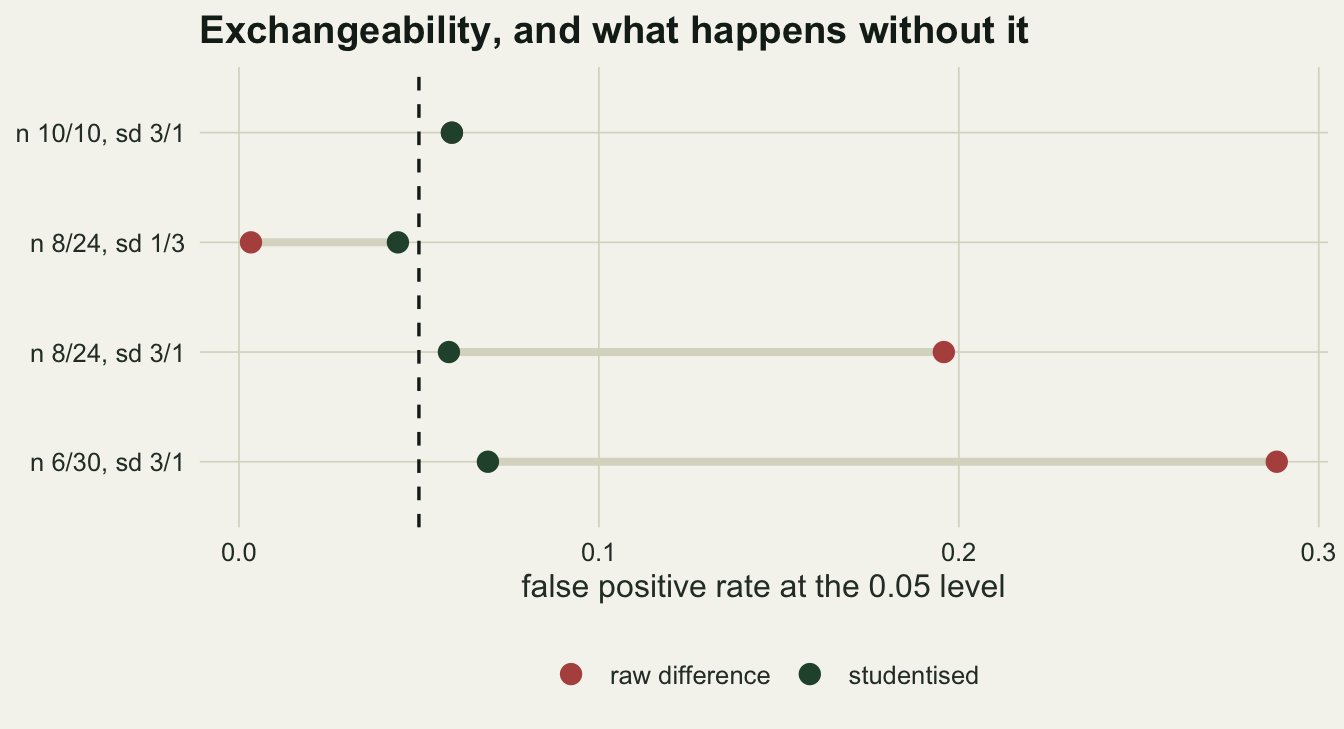
The pattern is the familiar one from the two-sample t test, arriving by a different route. A permutation test is not immune to unequal variances; it is immune to the shape of the distribution. Janssen showed in 1997 that the studentised permutation test keeps its level under the generalised Behrens-Fisher setting where the raw one does not, and this is what that result looks like on sixteen to thirty six plots.
What to report
Give the number of permutations next to every permutation p value. Without it the reader cannot tell whether 0.001 means a small p value or means the floor, and those are different claims.
Enumerate when you can. Under about twenty units in total the complete set of splits is a combn() call, the answer has no sampling error, and you learn the resolution of your own design for free.
Studentise the statistic when the groups differ in size, unless you have a reason to believe the spread is the same in both. With balanced groups it changes little; with a two to one imbalance it is the difference between a test with a level and a test without one.
Say which null hypothesis the shuffling encodes. “Treatment had no effect on any plot” and “the two means are equal” are different statements, and permutation tests the first.
Honest limits
Everything here is a two-sample comparison of means with unrestricted shuffling. Real ecological designs have blocks, split units, repeated measures and nested structure, and in those the choice of what may be exchanged with what is a larger source of error than anything measured above. That choice is covered on the site under PERMANOVA and under network null models, and the arithmetic in this post says nothing about it.
The studentised statistic is a repair, not a cure. At eight against twenty four it still rejects a true null slightly more often than the nominal rate, and the residual excess grows as the smaller group shrinks. There is no permutation statistic that makes a six against thirty comparison of unequal variances behave like a balanced one.
The exact enumeration here counts a split as extreme when its statistic is at least the observed one, with a numerical tolerance. Ties matter for discrete or heavily rounded data, where many splits give exactly the same statistic and the p value can jump by more than one rung of the ladder. Data recorded to two decimal places, as here, has essentially no ties; count data with a small range has many.
The false positive rates are estimated from 1200 datasets, so a rate near the nominal level carries a standard error of about 0.6 of a percentage point. The studentised rate at six against thirty sits 3.0 standard errors above nominal and is a real excess; the equal size comparison at 0.059 is not distinguishable from 0.05. The rank ordering of the four designs is not in doubt; the second decimal place of any one of them is.
Finally, none of this is an argument against permutation tests. The exact enumeration in this post is a complete, assumption-light answer that took milliseconds, and that is a good position to be in. The argument is against reading the word exact as covering the sampling step and the exchangeability assumption, neither of which it touches.
References
Ernst MD 2004 Statistical Science 19(4) (10.1214/088342304000000396)
Janssen A 1997 Statistics and Probability Letters 36(1):9-21 (10.1016/S0167-7152(97)00043-6)
Phipson B, Smyth GK 2010 Statistical Applications in Genetics and Molecular Biology 9(1) (10.2202/1544-6115.1585)