library(ggplot2)
library(patchwork)

te_paper  <- "#f5f4ee"
te_ink    <- "#16241d"
te_body   <- "#2c3a31"
te_forest <- "#275139"
te_rust   <- "#b5534e"
te_gold   <- "#c9b458"
te_line   <- "#dad9ca"

theme_datasheet <- function() {
  theme_minimal(base_size = 12) +
    theme(plot.background  = element_rect(fill = te_paper, colour = NA),
          panel.background = element_rect(fill = te_paper, colour = NA),
          panel.grid.major = element_line(colour = te_line, linewidth = 0.3),
          panel.grid.minor = element_blank(),
          text             = element_text(colour = te_body),
          plot.title       = element_text(colour = te_ink, face = "bold"),
          plot.subtitle    = element_text(colour = te_body),
          axis.text        = element_text(colour = te_body))
}Comparing two groups of angles
R
circular statistics
hypothesis testing
permutation tests
ecology tutorial
The Watson-Williams test fails on dispersed bearings, and permuting the angular gap does not repair it when mean resultant lengths are low, measured in base R.
Sixty birds are released one at a time from the same displacement site, thirty adults and thirty in their first autumn, and each is followed with binoculars until it disappears. Every bird contributes one number: the bearing at which it vanished. The adults leave in a tight cone. The juveniles scatter over most of the horizon. That age difference in scatter is the premise of the example rather than a claim about any particular species, and it is the feature the standard test cannot cope with.
The question the release was designed to answer is whether the two age classes head in different directions on average. That is a two-sample problem on the circle, and the standard answer is the Watson-Williams F test: a one line calculation that behaves like a one-way analysis of variance on the resultant lengths. It carries an assumption that textbooks state and papers rarely check. Both samples must come from von Mises distributions with the same concentration, and that concentration must be high. The juveniles have already broken the second half of it, and the age difference in scatter breaks the first.
The reflex when an assumption is doubtful is to permute: shuffle the age labels, recompute the statistic, count. In the linear world that reflex has a basis when the groups are the same size. A raw, unstudentised permutation test of the difference in two means is asymptotically level correct under unequal variances when the two groups have equal n, which is why the site’s permutation post can say that studentising changes an answer mainly when the group sizes differ. The result is asymptotic, though, and it turns on the shape of the two distributions as much as on their sizes. This post measures what survives of it at thirty per group, and then what happens to it on the circle.
What follows is a size study, not a power study: every rejection reported below is a false positive, because both groups are drawn with the same true mean direction throughout. The other circular posts on the site are one-sample or descriptive work: fitting a von Mises, testing a single sample against uniformity, checking what a circular summary hides. The post on activity patterns and temporal overlap does put two samples beside each other, but it compares whole distributions with a coefficient of overlap and a bootstrap interval rather than testing their mean directions against each other. No post on the site tests two mean directions, and the Watson-Williams test appears nowhere else. The one thing this post insists on is naming the statistic that gets permuted, because two reasonable choices give two different tests with two different false positive rates.
Sixty bearings and one true direction
The generating process is fixed and known. Both age classes have a mean direction of due north; only their concentrations differ, and any gap between the two sample mean directions is sampling noise.
Nothing here needs a circular package. The von Mises sampler is the rejection algorithm of Best and Fisher 1979, the mean direction is an atan2 of two sums, and the inverse of the ratio of Bessel functions that turns a mean resultant length into a concentration estimate is the piecewise approximation given by Fisher 1993.
rvm <- function(n, mu, kap) {
  aa <- 1 + sqrt(1 + 4 * kap^2)
  bb <- (aa - sqrt(2 * aa)) / (2 * kap)
  rr <- (1 + bb^2) / (2 * bb)
  out <- numeric(0)
  while (length(out) < n) {
    m  <- 2 * (n - length(out)) + 8
    u1 <- runif(m); u2 <- runif(m); u3 <- runif(m)
    zz <- cos(pi * u1)
    ff <- pmin(pmax((1 + rr * zz) / (rr + zz), -1), 1)
    cc <- kap * (rr - ff)
    keep <- (cc * (2 - cc) - u2 > 0) | (log(cc / u2) + 1 - cc >= 0)
    out <- c(out, ((mu + sign(u3 - 0.5) * acos(ff)) %% (2 * pi))[keep])
  }
  out[seq_len(n)]
}
mean_dir <- function(th) atan2(sum(sin(th)), sum(cos(th))) %% (2 * pi)
rbar_of  <- function(th) sqrt(sum(cos(th))^2 + sum(sin(th))^2) / length(th)
wrap_gap <- function(d) { d <- d %% (2 * pi); pmin(d, 2 * pi - d) }
in_deg   <- function(x) x * 180 / pi
a1inv <- function(x) ifelse(x < 0.53, 2 * x + x^3 + 5 * x^5 / 6,
                     ifelse(x < 0.85, -0.4 + 1.39 * x + 0.43 / (1 - x),
                            1 / (x^3 - 4 * x^2 + 3 * x)))

mu_home <- pi / 2
kap_ad  <- 4; kap_ju <- 0.8
n_ad    <- 30; n_ju  <- 30
set.seed(4014)
bear_ad <- rvm(n_ad, mu_home, kap_ad)
bear_ju <- rvm(n_ju, mu_home, kap_ju)

gap_deg <- in_deg(wrap_gap(mean_dir(bear_ad) - mean_dir(bear_ju)))
rb_ad   <- rbar_of(bear_ad); rb_ju <- rbar_of(bear_ju)
khat_ad <- a1inv(rb_ad); khat_ju <- a1inv(rb_ju)
The adults are drawn at concentration 4.0 and the juveniles at 0.8, both around due north. The adults return a mean resultant length of 0.84, which is a fitted concentration of 3.4, and the juveniles 0.26, a concentration of 0.53. The two sample mean directions sit 39.6 degrees apart, and the correct answer for this release is still that there is no difference to find. This particular release was picked from a run of simulated ones because it produces the failure the post is about: it is not typical, and how often it happens is measured further down.
ang  <- seq(0, 2 * pi, length.out = 240)
ring <- data.frame(x = cos(ang), y = sin(ang))
card <- data.frame(x = c(0, 1.24, 0, -1.24), y = c(1.24, 0, -1.24, 0),
                   lab = c("N", "E", "S", "W"))
compass_panel <- function(th, shade, ttl, note) {
  jr  <- 1 + (seq_along(th) %% 6) * 0.022
  pts <- data.frame(x = jr * cos(th), y = jr * sin(th))
  arw <- data.frame(xe = rbar_of(th) * cos(mean_dir(th)),
                    ye = rbar_of(th) * sin(mean_dir(th)))
  ggplot() +
    geom_path(data = ring, aes(x, y), colour = te_line, linewidth = 0.6) +
    geom_text(data = card, aes(x, y, label = lab), colour = te_body, size = 3.4) +
    geom_point(data = pts, aes(x, y), colour = shade, size = 1.8, alpha = 0.8) +
    geom_segment(data = arw, aes(x = 0, y = 0, xend = xe, yend = ye),
                 colour = te_ink, linewidth = 0.9,
                 arrow = arrow(length = unit(0.16, "cm"), type = "closed")) +
    coord_fixed(xlim = c(-1.45, 1.45), ylim = c(-1.45, 1.45)) +
    labs(title = ttl, subtitle = note) +
    theme_void(base_size = 12) +
    theme(plot.background  = element_rect(fill = te_paper, colour = NA),
          panel.background = element_rect(fill = te_paper, colour = NA),
          plot.title    = element_text(colour = te_ink, face = "bold", hjust = 0.5),
          plot.subtitle = element_text(colour = te_body, hjust = 0.5, size = 9))
}
(compass_panel(bear_ad, te_forest, "Adults", sprintf("mean resultant %.2f", rb_ad)) +
 compass_panel(bear_ju, te_gold, "Juveniles", sprintf("mean resultant %.2f", rb_ju))) +
  plot_annotation(theme = theme_datasheet())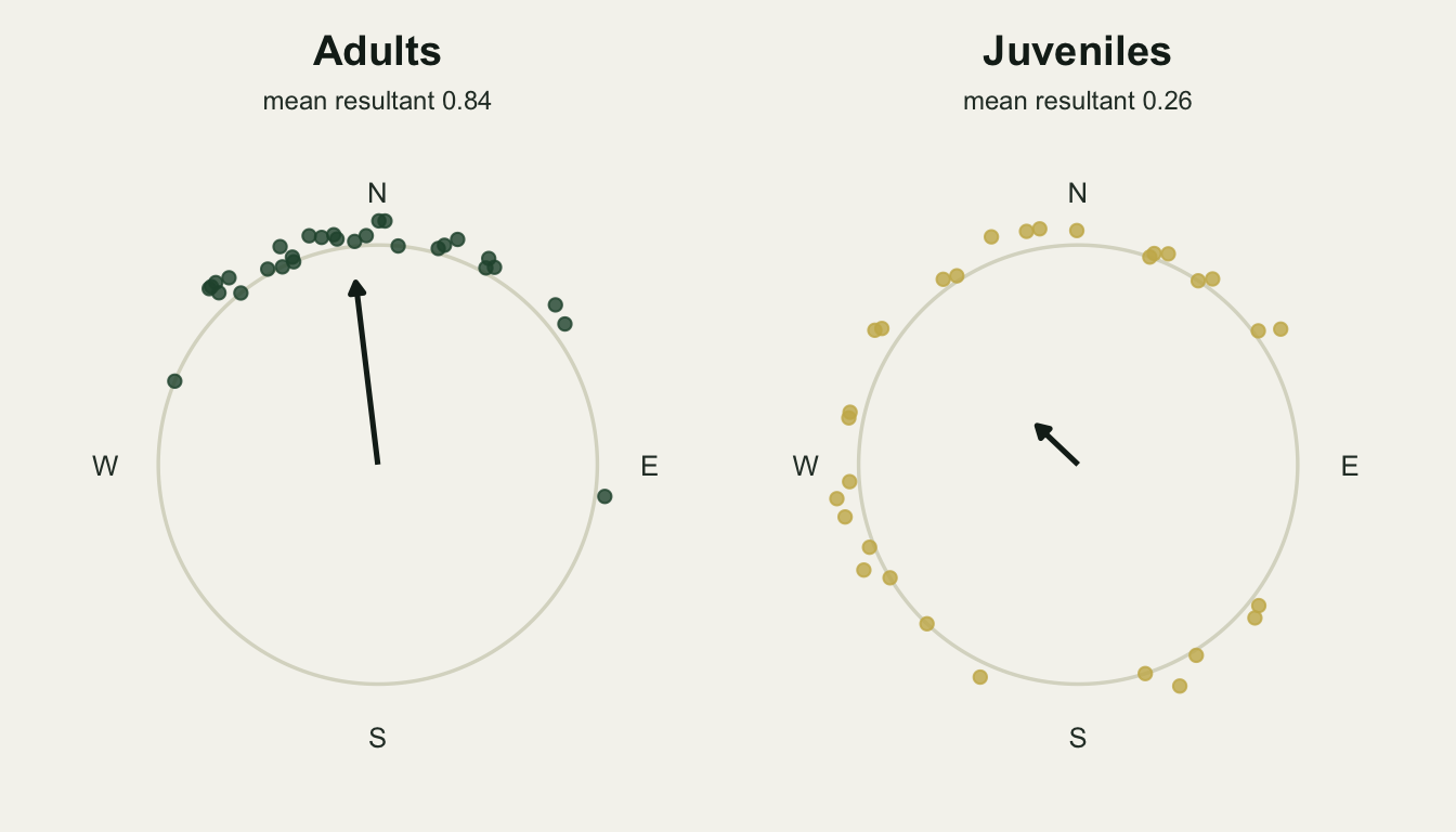
Naming the statistic is half the test
The Watson-Williams F statistic, from Watson and Williams 1956, compares the sum of the two within-group resultant lengths with the resultant length of the pooled sample. Write R1 and R2 for the group resultants and RT for the pooled one; then R1 + R2 - RT plays the part of a between-group sum of squares and N - R1 - R2 the part of a within-group one. The bracket in front is a small-sample correction that depends on a concentration estimated from the pooled mean resultant length.
Three permutation tests are then available, and they are not the same test.
The first permutes the angular distance between the two sample mean directions. That is the natural transposition of the raw difference in means, and it is the choice a reader who has met permutation tests on linear data will reach for.
The second permutes the Watson-Williams F statistic itself, treating F as a distance measure and letting the shuffling supply its null distribution rather than the F table.
The third permutes a studentised distance: the squared angular gap divided by an estimate of its own variance, where the variance of a sample mean direction is (1 - rho2) / (2 n rbar^2) with rho2 the second central trigonometric moment of that group. That is the quantity Fisher and Lewis 1983 use to combine mean directions with differing dispersions, and it is the circular counterpart of dividing by a standard error.
All three, plus the F table and a large-sample chi-squared reference for the studentised distance, come out of one function.
two_sample_p <- function(th1, th2, n_perm = 499) {
  n1 <- length(th1); n2 <- length(th2); nn <- n1 + n2
  th <- c(th1, th2)
  cv <- cos(th); sv <- sin(th); c2 <- cos(2 * th); s2 <- sin(2 * th)
  ct <- sum(cv); st <- sum(sv); c2t <- sum(c2); s2t <- sum(s2)
  r_tot <- sqrt(ct^2 + st^2)
  stats_of <- function(ca, sa, c2a, s2a) {
    cb <- ct - ca; sb <- st - sa; c2b <- c2t - c2a; s2b <- s2t - s2a
    ra <- sqrt(ca^2 + sa^2); rb <- sqrt(cb^2 + sb^2)
    m1 <- atan2(sa, ca); m2 <- atan2(sb, cb)
    kf <- 1 + 3 / (8 * a1inv((ra + rb) / nn))          # Stephens's correction
    d1 <- (1 - (cos(2 * m1) * c2a + sin(2 * m1) * s2a) / n1) / (2 * n1 * (ra / n1)^2)
    d2 <- (1 - (cos(2 * m2) * c2b + sin(2 * m2) * s2b) / n2) / (2 * n2 * (rb / n2)^2)
    cbind(gap  = wrap_gap(m1 - m2),
          ww   = kf * (nn - 2) * (ra + rb - r_tot) / (nn - ra - rb),
          stud = wrap_gap(m1 - m2)^2 / (d1 + d2))
  }
  obs <- drop(stats_of(sum(cv[1:n1]), sum(sv[1:n1]), sum(c2[1:n1]), sum(s2[1:n1])))
  idx <- replicate(n_perm, sample.int(nn, n1))
  pm  <- stats_of(colSums(matrix(cv[idx], n1)), colSums(matrix(sv[idx], n1)),
                  colSums(matrix(c2[idx], n1)), colSums(matrix(s2[idx], n1)))
  shuf <- (1 + colSums(sweep(pm, 2, obs, ">="))) / (n_perm + 1)
  c(ww_F      = unname(pf(obs[["ww"]], 1, nn - 2, lower.tail = FALSE)),
    perm_gap  = shuf[["gap"]],
    perm_F    = shuf[["ww"]],
    perm_stud = shuf[["stud"]],
    chisq     = unname(pchisq(obs[["stud"]], 1, lower.tail = FALSE)))
}

n_perm_rel <- 4999
set.seed(918)
p_rel <- two_sample_p(bear_ad, bear_ju, n_perm_rel)
round(p_rel, 4)
ww_F perm_gap perm_F perm_stud chisq
0.0559 0.0146 0.0410 0.1772 0.1813 On this release the F table returns 0.056, which just fails to reject. The permuted angular gap returns 0.0146 and the permuted F statistic 0.0410, so both permutation tests declare an age difference in heading that does not exist. The studentised permutation returns 0.177 and its large-sample chi-squared version 0.181, and both are right. Five procedures, one dataset, and a factor of 12 between the smallest and largest p value.
One dataset settles nothing. The rest of the post is the calibration study.
Watson-Williams needs a concentration field data rarely has
Start with the easy case: both groups drawn from the same concentration, so the only assumption in question is whether that concentration is high enough for the F approximation. Nominal level five per cent, thirty against thirty, seven concentrations, and a few thousand simulated releases in every cell.
alpha    <- 0.05
n_rep    <- 2000
kap_grid <- c(0.5, 0.75, 1, 1.5, 2, 3, 4)
size_cell <- function(ka, kb, reps, seed, n1 = 30, n2 = 30, n_perm = 399) {
  set.seed(seed)
  rowMeans(replicate(reps, two_sample_p(rvm(n1, mu_home, ka),
                                        rvm(n2, mu_home, kb), n_perm)) <= alpha)
}
size_eq <- t(vapply(seq_along(kap_grid),
                    function(i) size_cell(kap_grid[i], kap_grid[i], n_rep, 300 + i),
                    numeric(5)))
rownames(size_eq) <- sprintf("kappa %.2f", kap_grid)
se_rate  <- sqrt(alpha * (1 - alpha) / n_rep)
ww_low   <- size_eq[1, "ww_F"]
ww_mid   <- size_eq[3, "ww_F"]
ww_high  <- size_eq[7, "ww_F"]
ww_ratio <- ww_low / alpha
perm_worst <- max(abs(size_eq[, c("perm_gap", "perm_F")] - alpha)) / se_rate
round(size_eq, 3)
ww_F perm_gap perm_F perm_stud chisq
kappa 0.50 0.207 0.040 0.045 0.045 0.070
kappa 0.75 0.120 0.050 0.051 0.048 0.060
kappa 1.00 0.078 0.054 0.054 0.056 0.061
kappa 1.50 0.045 0.044 0.046 0.044 0.050
kappa 2.00 0.043 0.044 0.045 0.046 0.050
kappa 3.00 0.042 0.046 0.046 0.044 0.051
kappa 4.00 0.046 0.046 0.046 0.046 0.057At a concentration of 0.5, which is a mean resultant length near a quarter and an entirely ordinary figure for juvenile orientation, the Watson-Williams test rejects a true null 20.7 per cent of the time. That is 4.1 times the rate it advertises. At a concentration of 1.0 it is still 7.8 per cent, and only from about 1.5 upwards does it settle, reaching 4.6 per cent at the concentration of the adults. The usual textbook advice is to apply the test only when the mean resultant length exceeds about 0.7, and these rates are what that advice is protecting against.
Both permutation tests hold their level across the whole range: the largest departure from 0.05 over all fourteen cells is 2.1 standard errors, which is what fourteen honest estimates of a correct level would produce. With equal concentrations the labels really are exchangeable, and a permutation test under exchangeability does what it says.
size_long <- data.frame(
  kappa  = rep(kap_grid, 3),
  rate   = c(size_eq[, "ww_F"], size_eq[, "perm_gap"], size_eq[, "perm_F"]),
  method = rep(c("Watson-Williams F table", "permuted mean difference",
                 "permuted F statistic"), each = length(kap_grid)))
size_long$method <- factor(size_long$method,
  levels = c("permuted mean difference", "permuted F statistic",
             "Watson-Williams F table"))
ggplot(size_long, aes(kappa, rate, colour = method)) +
  geom_hline(yintercept = alpha, colour = te_ink, linetype = "dashed",
             linewidth = 0.6) +
  geom_line(linewidth = 0.9) +
  geom_point(size = 2.2) +
  scale_colour_manual(values = c(te_forest, te_gold, te_rust), name = NULL) +
  scale_y_continuous(limits = c(0, NA)) +
  labs(x = "concentration of both groups", y = "false positive rate",
       title = "Equal concentrations: only the F table misbehaves",
       subtitle = "dashed line: the nominal five per cent") +
  theme_datasheet() +
  theme(legend.position = "bottom")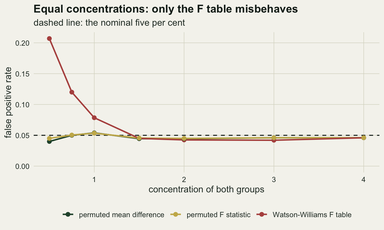
The free pass on the line is a property of the normal shape
The equal-n result is worth stating precisely, because the version that gets repeated is stronger than the version that is true. What holds is asymptotic: as n grows with the two groups the same size, the permutation distribution of the raw mean difference converges on the correct sampling distribution even when the two variances differ. At a finite n it is an approximation, and how good an approximation depends on the shape of the two distributions. The block below fixes the dispersion ratio at the value the circular pair will need and varies the shape of the more dispersed group, then fixes the shape and varies n, then fixes both and varies the ratio.
lin_perm <- function(draw_wide, draw_tight, n_each, n_perm) {
  v <- c(draw_wide(n_each), draw_tight(n_each))
  nn <- 2 * n_each; tot <- sum(v)
  gp <- function(sa) abs(sa / n_each - (tot - sa) / n_each)
  ob  <- gp(sum(v[1:n_each]))
  idx <- replicate(n_perm, sample.int(nn, n_each))
  (1 + sum(gp(colSums(matrix(v[idx], n_each))) >= ob - 1e-12)) / (n_perm + 1)
}
lin_rate <- function(dw, dt, n_each, seed, reps, n_perm) {
  set.seed(seed)
  mean(replicate(reps, lin_perm(dw, dt, n_each, n_perm)) <= alpha)
}
std_norm  <- function(s) function(k) rnorm(k, 0, s)          # centred, sd = s
std_exp   <- function(s) function(k) (rexp(k, 1) - 1) * s
std_lnorm <- function(s, w) function(k) {
  mid <- exp(w^2 / 2); spread <- sqrt((exp(w^2) - 1) * exp(w^2))
  (rlnorm(k, 0, w) - mid) / spread * s
}
csd_of    <- function(k) sqrt(-2 * log(besselI(k, 1) / besselI(k, 0)))
csd_ad    <- csd_of(kap_ad); csd_ju <- csd_of(kap_ju)
sd_ratio  <- csd_ju / csd_ad
n_rep_lin <- 3000; n_perm_lin <- 199; w_log <- 1.2; wide_sd <- 5
wide_draw  <- list(std_norm(sd_ratio), std_exp(sd_ratio),
                   std_lnorm(sd_ratio, w_log), std_norm(sd_ratio))
tight_draw <- list(std_norm(1), std_norm(1), std_norm(1), std_lnorm(1, w_log))
lin_shape <- vapply(seq_along(wide_draw), function(i)
  lin_rate(wide_draw[[i]], tight_draw[[i]], n_ad, 6100 + i, n_rep_lin, n_perm_lin),
  numeric(1))
n_grid <- c(5, 10, 30, 60)
lin_n  <- vapply(seq_along(n_grid), function(i)
  lin_rate(std_norm(wide_sd), std_norm(1), n_grid[i], 6200 + i, n_rep_lin, n_perm_lin),
  numeric(1))
rat_grid <- c(1, sd_ratio, wide_sd, 100)
lin_rat  <- vapply(seq_along(rat_grid), function(i)
  lin_rate(std_norm(rat_grid[i]), std_norm(1), n_ad, 6300 + i, n_rep_lin, n_perm_lin),
  numeric(1))
se_lin         <- sqrt(alpha * (1 - alpha) / n_rep_lin)
lin_big_n      <- max(abs(lin_n[3:4] - alpha)) / se_lin
lin_rat_spread <- (max(lin_rat) - min(lin_rat)) / se_lin
round(rbind(shape = lin_shape, size = lin_n, ratio = lin_rat), 4)
[,1] [,2] [,3] [,4]
shape 0.0497 0.0697 0.1053 0.0513
size 0.0760 0.0627 0.0500 0.0543
ratio 0.0507 0.0517 0.0537 0.0537With both groups normal at thirty each, the raw permutation test rejects 4.97 per cent of the time against a nominal 5.0 per cent, which is the free pass working as advertised. Replace the dispersed group with a centred exponential of the same standard deviation and the rate rises to 7.0 per cent; make it a centred lognormal instead and it reaches 10.5 per cent, 14 standard errors above nominal. Reverse the pairing, so that the skewed distribution is the tight group and the dispersed one is normal, and the rate drops back to 5.1 per cent. What breaks the test is not skewness somewhere in the data: it is skewness in the group that also carries the larger spread. The release at the top of this post is not that configuration: both age classes there are von Mises, symmetric about the same mean direction and differing only in concentration.
Sample size does the rest. With both groups normal and a 5 to one ratio of standard deviations, five per group rejects 7.6 per cent of the time and ten per group 6.3 per cent, while thirty and sixty per group sit within 1.1 standard errors of nominal. The asymptotics arrive early for normal data and late for skewed data, and thirty per group is early enough only in the first case.
The dispersion ratio itself does almost nothing. At thirty per group with both groups normal, standard deviation ratios of one, 2.60, 5 and 100 to one give rates spread over 0.8 standard errors, less than four independent estimates of a single number would usually scatter. That is the part to carry across: on the line, with equal group sizes and the same shape in both groups, how unequal the two variances are is not what decides whether the test holds its level.
The same dispersion ratio costs far more on the circle
Now make the two concentrations differ, which is the situation the release was built around. The linear study above was matched to it through dispersion: a von Mises with concentration 4.0 has a circular standard deviation of sqrt(-2 log(rbar)) radians, the same formula at concentration 0.8 gives a second value, and their ratio is the one the linear standard deviations were made to reproduce. That is the like-for-like a reader would build, and the section above is the reason to distrust it: the ratio was the one quantity on the line that made no difference. What does the work on the circle is identified in the next section.
n_rep_un <- 3000
circ_un  <- size_cell(kap_ad, kap_ju, n_rep_un, 8811, n_perm = 499)
se_un    <- sqrt(alpha * (1 - alpha) / n_rep_un)
round(circ_un, 4)
ww_F perm_gap perm_F perm_stud chisq
0.1203 0.1833 0.1393 0.0700 0.0737 The two circular standard deviations are 0.54 and 1.41 radians, a ratio of 2.60. On the circle that ratio gives 18.3 per cent for the permuted mean difference and 13.9 per cent for the permuted F statistic, against the 5.2 per cent it cost on the line at the same thirty against thirty. The Watson-Williams F table, which the permutation was supposed to improve on, gives 12.0 per cent. Permuting the natural statistic is the worst of the three, and it is worse than doing nothing.
The reason the two permutation tests differ is worth stating plainly, because it is the part that a description like “we used a permutation test” hides. The Watson-Williams F is a monotone function of the sum of the two within-group resultant lengths, since the pooled resultant and the sample size are the same for every shuffle. The angular gap between the two mean directions is not a function of that sum. The two statistics therefore rank the shuffles differently, and any p value computed from one of them is a different quantity from the p value computed from the other.
draw_circ <- function() c(rvm(30, mu_home, kap_ad), rvm(30, mu_home, kap_ju))
draw_lin  <- function() c(rnorm(30, 0, sd_ratio), rnorm(30, 0, 1))

gap_circ <- function(v, idx) {
  ca <- colSums(matrix(cos(v)[idx], 30)); sa <- colSums(matrix(sin(v)[idx], 30))
  in_deg(wrap_gap(atan2(sa, ca) - atan2(sum(sin(v)) - sa, sum(cos(v)) - ca)))
}
gap_lin <- function(v, idx) {
  sa <- colSums(matrix(v[idx], 30)); abs(sa / 30 - (sum(v) - sa) / 30)
}
pool_ref <- function(draw, gap_of, reps, n_perm) unlist(lapply(seq_len(reps),
  function(i) gap_of(draw(), replicate(n_perm, sample.int(60, 30)))))
n_ref_set  <- 1000
n_ref_perm <- 125
n_draw     <- 120000
one_split  <- matrix(seq_len(30))
set.seed(7001); ref_circ  <- pool_ref(draw_circ, gap_circ, n_ref_set, n_ref_perm)
set.seed(7002); null_circ <- replicate(n_draw, gap_circ(draw_circ(), one_split))
set.seed(7003); ref_lin   <- pool_ref(draw_lin, gap_lin, n_ref_set, n_ref_perm)
set.seed(7004); null_lin  <- replicate(n_draw, gap_lin(draw_lin(), one_split))

q_ref_circ  <- unname(quantile(ref_circ, 1 - alpha))
q_null_circ <- unname(quantile(null_circ, 1 - alpha))
q_ref_lin   <- unname(quantile(ref_lin, 1 - alpha))
q_null_lin  <- unname(quantile(null_lin, 1 - alpha))
q_ratio_circ <- q_ref_circ / q_null_circ

dens_panel <- function(refv, nullv, q_ref, q_null, x_lab, ttl) {
  dd <- data.frame(value = c(refv, nullv), origin = rep(
    c("permutation reference", "true null"), c(length(refv), length(nullv))))
  ggplot(dd, aes(value, colour = origin)) +
    geom_density(linewidth = 0.9) +
    geom_vline(xintercept = c(q_ref, q_null), linetype = "dashed",
               linewidth = 0.6, colour = c(te_rust, te_forest)) +
    scale_colour_manual(values = c(te_rust, te_forest), name = NULL) +
    labs(x = x_lab, y = "density", title = ttl) +
    theme_datasheet() + theme(legend.position = "bottom")
}

(dens_panel(ref_lin, null_lin, q_ref_lin, q_null_lin,
            "absolute difference in means", "On the line") +
 dens_panel(ref_circ, null_circ, q_ref_circ, q_null_circ,
            "angular gap (degrees)", "On the circle")) +
  plot_layout(guides = "collect") +
  plot_annotation(theme = theme_datasheet()) &
  theme(legend.position = "bottom")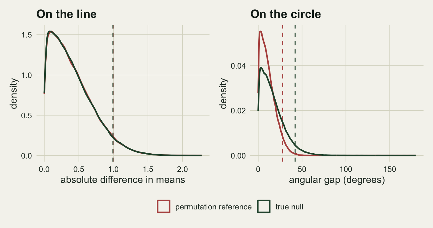
The figure is the whole argument in one picture. On the line the shuffled reference and the true sampling distribution have the same ninety fifth percentile, 1.00 against 0.99. On the circle the shuffled reference cuts off at 27.8 degrees while the statistic actually reaches 42.1 degrees under the null, a ratio of 0.66, so the critical value is about a third too small and the test rejects far too often. Fresh seeds move that ratio in the second decimal even at this many replicates, which is why it is not quoted more finely.
The mechanism is convexity, and the resultant length sets its size
Why the line escapes is arithmetic. The variance of a sample mean is the variance of one observation divided by n, and shuffling replaces two groups of thirty with two mixed groups each holding fifteen of each kind. The variance of a mixed group’s mean is the average of the two component variances divided by thirty, and the variance of the difference of two such means is that average times two over thirty, which is exactly the variance of the difference of the two unmixed means. Mixing averages the quantity that enters the variance, and the average is the same either way.
On the circle the quantity that enters is not the variance of an observation. The large-sample variance of a mean direction is (1 - rho2) / (2 n rbar^2), and shuffling averages rbar and rho2 separately across the two groups rather than averaging the ratio they sit in. Write a for the numerator 1 - rho2. What has to be true for the shuffled reference to be too narrow is that the pooled value of a / rbar^2 falls below the average of the two group values, and that does not follow from convexity of the reciprocal square on its own: the numerator moves too, and a / r^2 is not a jointly convex function of the pair.
The step that closes it for the von Mises family is that a falls as the resultant rises. The two numerators therefore act as weights that favour the dispersed group, and the comparison that has to come out right is against a resultant averaged with those weights rather than the plain average. Shuffling hands the test the plain average, which is the larger of the two. It is Jensen’s inequality with the weights supplied by the numerators, and both averages are in the chunk below.
a1_of   <- function(k) besselI(k, 1) / besselI(k, 0)
a2_of   <- function(k) besselI(k, 2) / besselI(k, 0)
var_dir <- function(r1, r2, n) (1 - r2) / (2 * n * r1^2)
shrink_of <- function(k1, k2, n) sqrt(
  2 * var_dir((a1_of(k1) + a1_of(k2)) / 2, (a2_of(k1) + a2_of(k2)) / 2, n) /
    (var_dir(a1_of(k1), a2_of(k1), n) + var_dir(a1_of(k2), a2_of(k2), n)))
aw <- c(1 - a2_of(kap_ad), 1 - a2_of(kap_ju))
r_unw <- mean(c(a1_of(kap_ad), a1_of(kap_ju)))
r_wgt <- sum(aw * c(a1_of(kap_ad), a1_of(kap_ju))) / sum(aw)
g_side   <- 400
k_grid   <- exp(seq(log(0.05), log(50), length.out = g_side))
shr_grid <- outer(k_grid, k_grid, shrink_of, n = n_ad)
off_diag <- shr_grid[row(shr_grid) != col(shr_grid)]
grid_max  <- max(off_diag)
grid_bad  <- sum(off_diag >= 1)
grid_ones <- sum(diag(shr_grid) == 1)
sd_shrink <- shrink_of(kap_ad, kap_ju, n_ad)
pred_size <- 2 * (1 - pnorm(qnorm(1 - alpha / 2) * sd_shrink))
n_big     <- 100
n_rep_big <- 800
circ_100  <- size_cell(kap_ad, kap_ju, n_rep_big, 9902, n1 = n_big, n2 = n_big,
                       n_perm = 499)
se_big    <- sqrt(alpha * (1 - alpha) / n_rep_big)
round(c(weighted_r = r_wgt, plain_r = r_unw, grid_at_or_above_one = grid_bad,
        shrink = sd_shrink, predicted = pred_size, circ_100), 4)
weighted_r plain_r grid_at_or_above_one
0.5275 0.6173 0.0000
shrink predicted ww_F
0.6983 0.1711 0.1175
perm_gap perm_F perm_stud
0.1775 0.1437 0.0562
chisq
0.0525 For the two concentrations used here the weighted average of the resultants is 0.527 and the plain average is 0.617, so the shuffled denominator is the larger one and the shuffled variance is the smaller. That argument is a statement about the von Mises family rather than about circular distributions in general, and it is not proved here. It was checked numerically instead, over a 400 by 400 grid of concentration pairs running from 0.05 to 50: the shrinkage factor came out below one at every one of the 159600 pairs with unequal concentrations, its largest value being 0.999999, and it was exactly one at all 400 points on the diagonal.
The same algebra predicts a shuffled reference distribution 0.698 times as wide as the true one, and feeding that through a normal approximation gives a predicted false positive rate of 0.171 for the permuted mean difference. It is checked against the measured rate a few paragraphs down, where two independent runs of the cell are available. The percentile ratio in the figure, 0.66, is a tighter number than 0.698, and the two are not required to agree: a ratio of ninety fifth percentiles equals a ratio of standard deviations only when the two distributions have the same shape, and wrapping a difference of angles onto half a circle means that a change of width is also a change of shape. Which way that pushes the percentile ratio is not something the closed form pins down.
Nothing in that calculation involves the sample size: the shrinkage factor is a ratio of variances and n cancels. So the distortion is not a small-sample artefact, and raising n should leave it where it is. At 100 against 100 the permuted mean difference rejects 17.8 per cent of the time, the permuted F statistic 14.4 per cent and the Watson-Williams F table 11.8 per cent. Raising both groups from thirty birds to a hundred left all three where they were. A test with the wrong level does not improve with effort.
What the shrinkage factor does involve is the concentration. Hold the dispersion ratio at the value used all the way through this post and slide both concentrations up together, and the factor climbs towards one, which is the same as saying the shuffled reference stops being too narrow. That is a prediction with a sweep attached to it.
conc_anchor <- c(2, 4, 8, 15, 40)
conc_mate   <- vapply(conc_anchor, function(kh) uniroot(
  function(kl) csd_of(kl) / csd_of(kh) - sd_ratio, c(1e-4, kh), tol = 1e-10)$root,
  numeric(1))
n_rep_conc  <- 2500
conc_rate   <- t(vapply(seq_along(conc_anchor), function(i)
  size_cell(conc_anchor[i], conc_mate[i], n_rep_conc, 7700 + i, n_perm = 499),
  numeric(5)))
conc_shrink <- shrink_of(conc_anchor, conc_mate, n_ad)
conc_pred   <- 2 * (1 - pnorm(qnorm(1 - alpha / 2) * conc_shrink))
conc_rb     <- a1_of(conc_mate)
se_conc     <- sqrt(alpha * (1 - alpha) / n_rep_conc)
pool_n    <- n_rep_un + n_rep_conc
pool_gap  <- (n_rep_un * circ_un[["perm_gap"]] + n_rep_conc * conc_rate[2, 2]) / pool_n
se_pool   <- sqrt(pool_gap * (1 - pool_gap) / pool_n)
pool_z    <- (pool_gap - pred_size) / se_pool
round(cbind(kappa = conc_anchor, mate = conc_mate, rbar = conc_rb,
            shrink = conc_shrink, predicted = conc_pred, conc_rate), 4)
kappa mate rbar shrink predicted ww_F perm_gap perm_F perm_stud
[1,] 2 0.1765 0.0879 0.2903 0.5694 0.4140 0.5116 0.3636 0.2004
[2,] 4 0.8000 0.3711 0.6983 0.1711 0.1180 0.1752 0.1344 0.0676
[3,] 8 1.6732 0.6361 0.8662 0.0895 0.0612 0.0916 0.0848 0.0560
[4,] 15 2.7763 0.7920 0.9295 0.0685 0.0488 0.0640 0.0632 0.0540
[5,] 40 6.3901 0.9180 0.9733 0.0564 0.0524 0.0520 0.0516 0.0496
chisq
[1,] 0.2104
[2,] 0.0708
[3,] 0.0596
[4,] 0.0560
[5,] 0.0592The second row of that table is the pair the whole post has been using, run again under a fresh seed. Pooling it with the earlier run gives 5500 releases and a rate of 0.180 for the permuted mean difference, against the predicted 0.171: a gap of 1.6 standard errors, which is agreement rather than disagreement. The closed form is doing real work here, not decoration.
Across the sweep the dispersion ratio is constant and the rate is not. Where the dispersed group has a mean resultant length of 0.09, the permuted mean difference rejects a true null 51 per cent of the time, and every procedure in the post is broken there, the studentised one included at 20 per cent. By a dispersed-group resultant of 0.64 the permuted mean difference is down to 9.2 per cent, and by 0.92 it is 5.2 per cent, within 0.5 standard errors of nominal. The free pass is not lost on the circle as such. It is lost when the mean resultant lengths are low, and it comes back when they are high, at a dispersion ratio that never changed.
That is the practical reading of the whole post. A reader whose animals are well oriented, with both groups above a mean resultant length of roughly 0.79, can permute the angular gap and be close enough to right at the dispersion ratio used throughout this post, which is the only unequal ratio measured on the circle here. A reader whose scattered group sits near a resultant of 0.37, an ordinary figure for juvenile orientation, cannot.
conc_long <- data.frame(
  rbar   = rep(conc_rb, 3),
  rate   = c(conc_rate[, "ww_F"], conc_rate[, "perm_gap"], conc_rate[, "perm_F"]),
  method = rep(c("Watson-Williams F table", "permuted mean difference",
                 "permuted F statistic"), each = length(conc_rb)))
conc_long$method <- factor(conc_long$method,
  levels = c("permuted mean difference", "permuted F statistic",
             "Watson-Williams F table"))
ggplot(conc_long, aes(rbar, rate, colour = method)) +
  geom_line(data = data.frame(rbar = conc_rb, rate = conc_pred),
            aes(rbar, rate), inherit.aes = FALSE, colour = te_line,
            linewidth = 3.4, lineend = "round") +
  geom_hline(yintercept = alpha, colour = te_ink, linetype = "dashed",
             linewidth = 0.6) +
  geom_line(linewidth = 0.9) +
  geom_point(size = 2.2) +
  scale_colour_manual(values = c(te_forest, te_gold, te_rust), name = NULL) +
  scale_y_continuous(limits = c(0, NA)) +
  labs(x = "mean resultant length of the dispersed group",
       y = "false positive rate",
       title = "Same dispersion ratio, five different concentrations",
       subtitle = "dashed line: nominal five per cent; pale band: closed-form prediction") +
  theme_datasheet() +
  theme(legend.position = "bottom")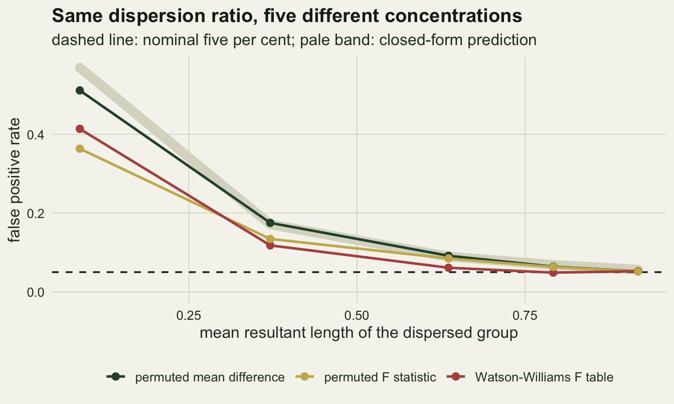
A studentised statistic recovers most of the level
The repair is the same one Janssen 1997 established for the linear Behrens-Fisher problem: divide by an estimate of the statistic’s own variance before permuting, so that the shuffled statistic is standardised inside every shuffle and the shrinkage cancels. On the circle the divisor is the sum of the two estimated mean direction variances, which is the third statistic already inside two_sample_p().
proc_lab <- c(ww_F = "Watson-Williams F table",
             perm_gap = "permuted mean difference",
             perm_F = "permuted F statistic",
             perm_stud = "permuted studentised gap",
             chisq = "large-sample chi-squared")
repair <- data.frame(
  method = rep(unname(proc_lab), 2),
  n_each = rep(c(n_ad, n_big), each = length(proc_lab)),
  rate   = c(circ_un[names(proc_lab)], circ_100[names(proc_lab)]))
repair$method <- factor(repair$method, levels = rev(unname(proc_lab)))
stud_30  <- circ_un[["perm_stud"]]
stud_100 <- circ_100[["perm_stud"]]
chi_100  <- circ_100[["chisq"]]
chi_low  <- size_eq[1, "chisq"]
round(repair$rate, 4)
[1] 0.1203 0.1833 0.1393 0.0700 0.0737 0.1175 0.1775 0.1437 0.0562 0.0525The studentised permutation test rejects 7.0 per cent of the time at thirty against thirty and 5.6 per cent at 100 against 100, and the large-sample chi-squared reference gives 5.2 per cent at the larger size. The repair is asymptotic, not exact: at thirty per group it still carries an excess of about 2.0 percentage points, which is 5.0 standard errors, and it is not free at the other end of the concentration range either. Where both groups are heavily dispersed, at a concentration of 0.5, the chi-squared version rejects 7.0 per cent of the time, because the variance formula it divides by is itself a large-sample approximation.
ggplot(repair, aes(rate, method, colour = factor(n_each))) +
  geom_vline(xintercept = alpha, colour = te_ink, linetype = "dashed",
             linewidth = 0.6) +
  geom_line(aes(group = method), colour = te_line, linewidth = 1.3) +
  geom_point(size = 3.2) +
  scale_colour_manual(values = c(te_gold, te_forest), name = "birds per group") +
  scale_x_continuous(limits = c(0, NA)) +
  labs(x = "false positive rate", y = NULL,
       title = "Concentration 4 against 0.8, same true direction",
       subtitle = "dashed line: the nominal five per cent") +
  theme_datasheet() +
  theme(legend.position = "bottom")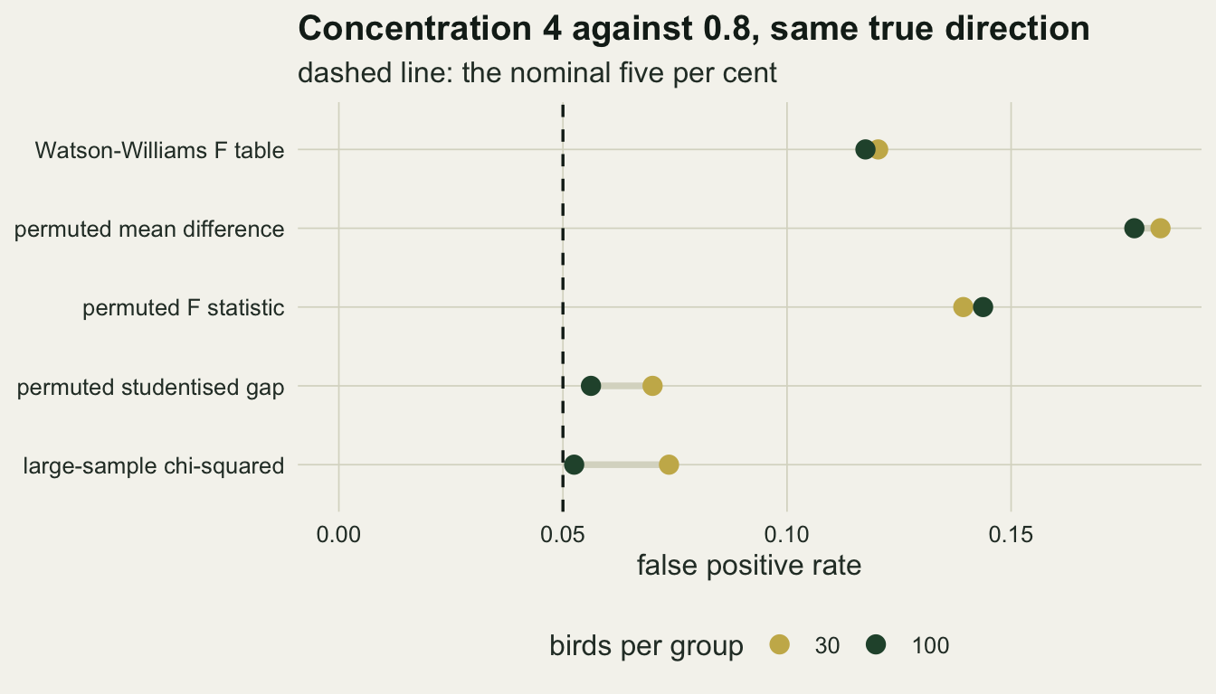
What to report
Give the mean resultant length of each group before giving any test of mean direction. It is one line of arithmetic, it is the quantity every assumption in this area is stated in terms of, and a reader who sees 0.26 for one group and 0.84 for the other knows immediately that the Watson-Williams test is out of its range.
Name the statistic that was permuted. “A permutation test with 999 shuffles” describes at least three different tests here, and at the concentrations used above they differ by 11 percentage points of false positive rate. The phrase is not a method; the statistic is.
If the two groups differ in concentration and the question is about mean direction, use a studentised statistic, either permuted or referred to a chi-squared distribution, and say which. If they do not differ, the plain permutation test is fine and the F table is fine too once the mean resultant length is above about 0.7.
Report the concentration difference as a result in its own right. In the release above, the age difference in scatter is real and the age difference in heading is not, and the second is the question only because the first was treated as a nuisance. Landler, Ruxton and Malkemper 2021 sort the two-sample circular literature along the same seam: they classify eighteen tests by whether the null being tested is identical distributions, equal mean directions or equal concentrations, and report that only eight of the eighteen held their nominal type one error rate across their simulations. The Watson-Williams test was not among the eight, and their recommendation for a general two-sample comparison is Watson’s U squared or a MANOVA on the trigonometric moments.
Say how many shuffles were used and give the resulting p value with its resolution, exactly as for any Monte Carlo test.
Honest limits
Everything above is measured under one alternative, which is no alternative at all: both groups always share a true mean direction, so every number is a size, not a power. A test that rejects too often is not thereby more powerful, and the studentised statistic pays for its level somewhere. That price is not measured here, and a full comparison would need a grid of true mean direction differences crossed with the concentration pairs.
The distributions are von Mises throughout, and the permutation tests are being asked to survive a difference in concentration only. Real bearing data is often a mixture: a directed component plus a scattered one, or a bimodal axis. A mixture breaks the von Mises assumption behind the variance formula as well, and the studentised statistic has no protection against that, since its divisor is estimated from the same second trigonometric moment that the mixture distorts.
The variance formula for a mean direction, and therefore the studentised statistic and the chi-squared reference, are large-sample results. The measured excess of 2.0 percentage points at thirty per group is what that costs at a size ecologists actually have, and the 7.0 per cent at the lowest concentration in the equal-concentration study is what it costs when the mean resultant length is small. Neither is a disaster and neither is nothing.
The simulation sizes are modest by design: 2000 releases per cell in the concentration curve, 3000 in the unequal-concentration cell, 2500 per cell in the concentration sweep, 3000 per linear cell and 800 at 100 per group. Those give standard errors of about 0.5, 0.4, 0.4, 0.4 and 0.8 of a percentage point for a rate sitting at the nominal five per cent, which is the wrong figure for the rates this post spends most of its time on. At the 18.3 per cent the permuted mean difference reaches at thirty per group the standard error is 0.7 of a percentage point, and at 100 per group it is 1.4. The ordering of the procedures is not in question at that precision; the second decimal of any single rate is.
A bootstrap that resamples within each group, rather than shuffling across them, is the other repair worth knowing about, because it never mixes the two concentrations in the first place. It is not measured here, and claiming it works without measuring it would be exactly the mistake this post is about.
References
Watson GS, Williams EJ 1956 Biometrika 43(3-4):344-352 (10.1093/biomet/43.3-4.344)
Best DJ, Fisher NI 1979 Applied Statistics 28(2):152-157 (10.2307/2346732)
Fisher NI, Lewis T 1983 Biometrika 70(2):333-341 (10.1093/biomet/70.2.333)
Janssen A 1997 Statistics and Probability Letters 36(1):9-21 (10.1016/S0167-7152(97)00043-6)
Landler L, Ruxton GD, Malkemper EP 2021 Scientific Reports 11(1):20337 (10.1038/s41598-021-99299-5)
Fisher NI 1993 Statistical Analysis of Circular Data. Cambridge University Press. ISBN 978-0-521-35018-1.