Hierarchical clustering and dendrograms in R

Turn a dissimilarity matrix into groups with hclust: a dendrogram, a linkage choice, a cut into clusters, and what that cut can and cannot prove about them.

An ordination like NMDS draws a continuous map: sites that sit close together have similar communities, and there are no hard borders. Hierarchical clustering takes the same dissimilarity information and does the opposite, carving the sites into discrete, nested groups and drawing the result as a tree. The two are complementary. Clustering is what you reach for when the question is “how many community types are here, and which site belongs to which?” rather than “how do communities grade into one another?”

This post builds a dendrogram in R from a Bray-Curtis dissimilarity matrix using hclust, walks through choosing a linkage method, cuts the tree into groups, and then checks those groups against an NMDS ordination of the same sites. That last step is worth being careful about: the ordination reads the same dissimilarity matrix the tree does, so agreement between them is a consistency check on the display, not evidence that the groups are real.

The ingredients

Hierarchical agglomerative clustering needs two decisions. The first is the dissimilarity between sites, which for community abundance data is usually Bray-Curtis (Bray and Curtis 1957), computed with vegan::vegdist. The second is the linkage rule, which decides how the distance between two groups of sites is measured once sites start merging. hclust then repeatedly fuses the two closest groups, from individual sites up to one tree.

A worked example

Here is a synthetic survey of 24 sites belonging to three community types, eight sites each. Types A and B share part of their species pool, so they should resemble each other more than either resembles C. The data is synthetic and illustrative.

library(vegan)
library(factoextra)
library(ggplot2)
te_canvas <- theme(plot.background  = element_rect(fill = "#f5f4ee", colour = NA),
                   panel.background = element_rect(fill = "#f5f4ee", colour = NA))
library(dplyr)

set.seed(5)
types <- rep(c("A", "B", "C"), each = 8)
n_sites <- length(types); Sp <- 26

mean_mat <- matrix(0.4, nrow = n_sites, ncol = Sp)
for (i in seq_len(n_sites)) {
  t <- types[i]
  if (t == "A") mean_mat[i, 1:8]   <- 8     # A: species 1-8
  if (t == "B") mean_mat[i, 5:12]  <- 8     # B: species 5-12 (overlaps A)
  if (t == "C") mean_mat[i, 17:26] <- 8     # C: species 17-26 (distinct)
  mean_mat[i, ] <- mean_mat[i, ] * runif(Sp, 0.7, 1.3)
}
comm <- matrix(rpois(n_sites * Sp, mean_mat), nrow = n_sites)
rownames(comm) <- paste0(types, ave(seq_len(n_sites), types, FUN = seq_along))
colnames(comm) <- paste0("sp", seq_len(Sp))

bc     <- vegdist(comm, method = "bray")
hc_avg <- hclust(bc, method = "average")

The dendrogram below is read vertically. Each leaf is a site; the height at which two branches join is the Bray-Curtis dissimilarity at which those groups fuse. Low joins mean very similar sites; the high join near the top is the most distinct split in the data.

clusters    <- cutree(hc_avg, k = 3)
# one colour per cluster, reused in the ordination below for consistency
clust_cols  <- c("1" = "#c98a2e", "2" = "#3a7ca5", "3" = "#275139")
lr_order    <- unique(clusters[hc_avg$order])   # cluster order, left to right in the tree

fviz_dend(hc_avg, k = 3, k_colors = clust_cols[as.character(lr_order)],
          color_labels_by_k = TRUE, lwd = 0.8, cex = 0.62, rect = FALSE,
          main = "", ylab = "Bray-Curtis dissimilarity",
          ggtheme = theme_minimal(base_size = 12) + te_canvas) +
  scale_x_continuous(breaks = NULL) +
  theme(panel.grid.major.x = element_blank(),
        axis.text.x = element_blank(), axis.ticks.x = element_blank())

Figure 1: The tree recovers the planted design, and the relationship as well: A and B fuse far below the height at which C joins them.

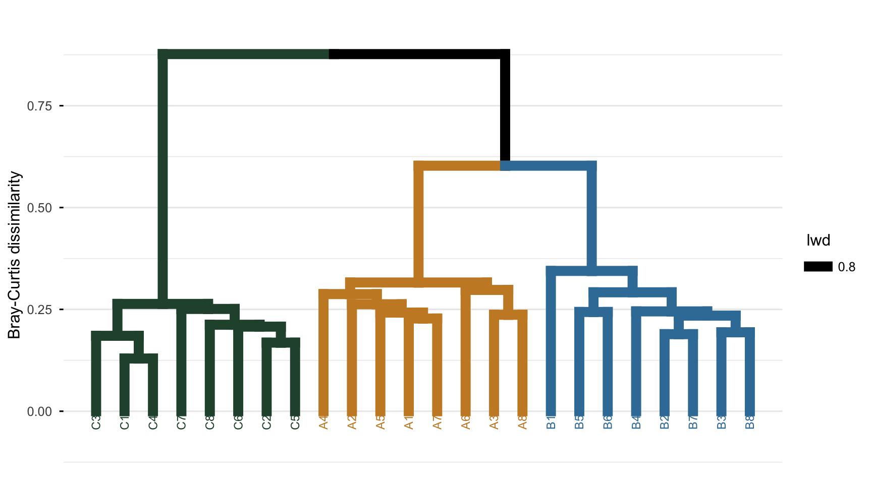
The structure matches the design. The C sites form one cluster that stays separate until the very top, while A and B fuse with each other at a much lower height before joining C. The tree has recovered not just three groups but their relationship: A and B are sibling types within a broader division from C, which is exactly how the species pools were built.

Choosing a linkage

The linkage rule changes the shape of the tree, sometimes dramatically, so it is worth knowing what the common choices do. Single linkage measures group distance by the closest pair of members, which tends to produce straggly, chained clusters. Complete linkage uses the farthest pair, producing tight compact clusters. Average linkage (UPGMA) uses the mean distance between groups and sits between the two. Ward’s method (Ward 1963) merges the groups that least increase within-cluster variance, often giving clean, roughly equal-sized clusters.

There is a quantitative way to compare them: the cophenetic correlation (Sokal and Rohlf 1962), the correlation between the original dissimilarities and the distances implied by the tree. A higher value means the dendrogram distorts the real distances less.

linkages <- c("average", "complete", "single", "ward.D2")
coph <- sapply(linkages, function(m) cor(bc, cophenetic(hclust(bc, method = m))))
round(sort(coph, decreasing = TRUE), 3)

 average  ward.D2   single complete 
   0.986    0.984    0.981    0.976 

For this dataset, average linkage preserves the distances best, which is common for Bray-Curtis community data and a reasonable default. It is not a universal rule: cophenetic correlation rewards faithfulness to the raw distances, while Ward’s method is often preferred when you specifically want compact, interpretable groups even at a small cost in fidelity. One R-specific trap is worth flagging: hclust offers both "ward.D" and "ward.D2", and only "ward.D2" implements Ward’s actual variance criterion on a distance matrix. Use "ward.D2" unless you have a particular reason not to.

Cutting the tree

A dendrogram on its own does not assign sites to groups; you have to cut it at some height, or equivalently ask for a fixed number of clusters with cutree. Cutting this tree into three recovers the planted types cleanly.

table(type = types, cluster = cutree(hc_avg, k = 3))

    cluster
type 1 2 3
   A 8 0 0
   B 0 8 0
   C 0 0 8

Choosing the number of clusters is the genuinely subjective part. The height of the joins is one guide: a long vertical gap before the next merge suggests a natural stopping point. Interpretability is another: clusters should correspond to something you can name. The check that carries real weight is an external one: groups predicted by the design, or by a variable that played no part in building the dissimilarity.

Cross-checking with NMDS

If the clusters are real structure rather than artefacts of the cutting, they should hold up as coherent regions in an ordination that was computed independently. Here is an NMDS of the same sites, with points coloured by their dendrogram cluster and shaped by their true type.

set.seed(5)
nmds <- metaMDS(comm, distance = "bray", k = 2, trymax = 50, trace = 0)

scores_df <- as.data.frame(scores(nmds, display = "sites"))
scores_df$site    <- rownames(scores_df)
scores_df$cluster <- factor(clusters[scores_df$site])
scores_df$type    <- types[match(scores_df$site, rownames(comm))]
hulls <- scores_df %>% group_by(cluster) %>% slice(chull(NMDS1, NMDS2))

ggplot(scores_df, aes(NMDS1, NMDS2, color = cluster)) +
  geom_polygon(data = hulls, aes(fill = cluster, group = cluster), alpha = 0.12, color = NA) +
  geom_point(aes(shape = type), size = 3, stroke = 1) +
  scale_color_manual(values = clust_cols, name = "cluster") +
  scale_fill_manual(values = clust_cols, guide = "none") +
  scale_shape_manual(values = c(A = 16, B = 17, C = 15), name = "true type") +
  annotate("text", x = Inf, y = -Inf, label = paste0("stress = ", round(nmds$stress, 3)),
           hjust = 1.1, vjust = -0.8, size = 3.2, color = "#5d6b61") +
  theme_minimal(base_size = 12) + te_canvas + theme(legend.position = "right")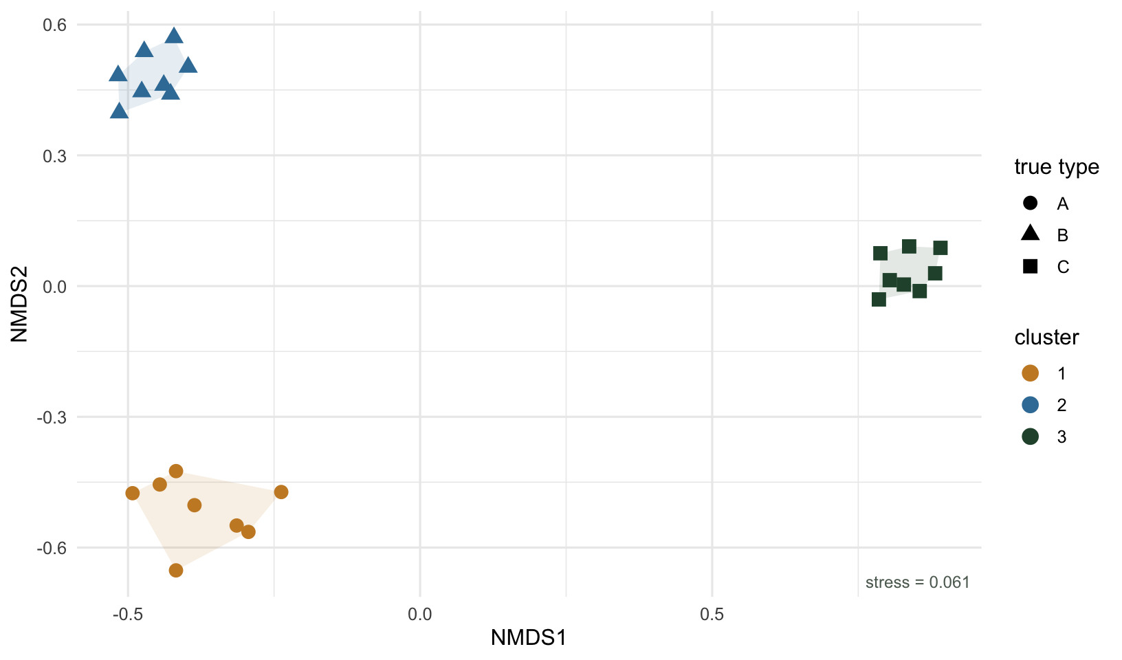

Figure 2: Colour is the dendrogram cluster, shape the true type. Two displays of the same dissimilarity matrix agree, which shows the cut is not an artefact of the linkage, and here the clusters also line up with the true types.

The three clusters land as three separate clouds, and within each cloud every point carries the same true-type shape. The dendrogram and the ordination, built from the same dissimilarities but displayed in completely different ways, tell the same story. That agreement says the cut survives a change of display; it is the match with the true type, which came from outside the dissimilarity matrix, that says the grouping is real. When clustering and ordination disagree, usually a cluster that the tree splits but the ordination shows as a single smear, it is a sign to revisit the number of clusters or the linkage.

Caveats

Hierarchical clustering will always return clusters, even when the data is a structureless cloud. The method cannot tell you whether groups exist, only how it would carve the data if they did. Treat the dendrogram as a hypothesis, and be careful how you test it. Running ANOSIM or PERMANOVA on the groups the tree just cut, using the dissimilarity the tree was built from, tests the data against itself, and it is worth measuring what that costs.

set.seed(11)
circular_p <- replicate(200, {
  noise <- matrix(rpois(30 * 20, lambda = 5), nrow = 30)   # no structure at all
  d     <- vegdist(noise, method = "bray")
  grp   <- factor(cutree(hclust(d, method = "average"), k = 2))
  adonis2(d ~ grp, permutations = 199)$`Pr(>F)`[1]
})
c(mean_p = round(mean(circular_p), 4),
  proportion_significant = mean(circular_p < 0.05))

                mean_p proportion_significant 
                0.0353                 0.7400 

Thirty sites of pure Poisson noise, cut into two clusters and then tested with the dissimilarity that produced the cut: 74 per cent of those structureless data sets come back significant at the five per cent level, on a mean p of 0.035. The exact rate moves with the number of sites, the number of species, the linkage and the cut, but it never lands anywhere near the nominal five per cent, because a test of the groups against the matrix that made them cannot fail. The cophenetic correlation does not rescue it either, since it measures how faithfully the tree preserves the distances, not whether groups exist. What does work is a null that includes the clustering step (recluster inside every permutation), a split-half check (find the groups on one half of the species, test them on the other), or groups that come from the design or from a variable outside the matrix.

The number of clusters is a decision, not an output. Different cut heights give different group counts, and there is rarely one correct answer; report how you chose and check that the conclusion is stable across reasonable alternatives.

The linkage and the dissimilarity both shape the result, so state them. The same sites under single linkage and Ward’s method can produce visibly different trees. And as always with Bray-Curtis on raw abundances, a few hyperabundant species can dominate the dissimilarities; if that is a concern, transform the data (a square-root or a Hellinger transformation) before clustering.

References

Bray JR, Curtis JT 1957 Ecological Monographs 27(4):325-349 (10.2307/1942268)

Legendre P, Legendre L 2012 Numerical Ecology, 3rd English edition, Elsevier (ISBN 978-0-444-53868-0)

Sokal RR, Rohlf FJ 1962 Taxon 11(2):33-40 (10.2307/1217208)

Ward JH Jr 1963 Journal of the American Statistical Association 58(301):236-244 (10.1080/01621459.1963.10500845)

Related tutorials

• Common PERMANOVA mistakes
• Checking a community classification
• Pairwise PERMANOVA
• Indicator species analysis