Checking a community classification

Cluster the sites, cut the dendrogram, then test the clusters with PERMANOVA on the same matrix: pure noise passes almost every time. A calibrated null in R.

The workflow is everywhere in community ecology. Compute a dissimilarity matrix, cluster the sites, cut the dendrogram into two or three groups, then run adonis2 or anosim to confirm that the groups differ. The confirmation almost always arrives.

It arrives because the groups were built from the same distances the test then examines. The clustering algorithm searched for the split that separates the sites best; the test asks whether the sites are separated. There is no data set on which that question can be answered no, so a significant result carries no information about whether the classification describes anything real.

This post measures how often the shortcut declares victory on data with no groups in it, shows why published rates for this failure disagree with each other, and builds a null that puts the clustering step inside the permutation, which is the fix.

Data with nothing in it

Thirty sites, twenty species, independent Poisson counts with the same mean everywhere. There are no groups, no gradient and no structure of any kind.

library(vegan)
library(ggplot2)

te_paper  <- "#f5f4ee"
te_ink    <- "#16241d"
te_body   <- "#2c3a31"
te_forest <- "#275139"
te_rust   <- "#b5534e"
te_gold   <- "#c9b458"
te_line   <- "#dad9ca"

theme_datasheet <- function() {
  theme_minimal(base_size = 12) +
    theme(plot.background  = element_rect(fill = te_paper, colour = NA),
          panel.background = element_rect(fill = te_paper, colour = NA),
          panel.grid.major = element_line(colour = te_line, linewidth = 0.3),
          panel.grid.minor = element_blank(),
          text             = element_text(colour = te_body),
          plot.title       = element_text(colour = te_ink, face = "bold"),
          axis.text        = element_text(colour = te_body))
}

n_site <- 30
n_sp   <- 20
noise_matrix <- function(n = n_site, p = n_sp, lambda = 5) {
  matrix(rpois(n * p, lambda), n, p)
}
cut_two <- function(d, linkage = "ward.D2") cutree(hclust(d, method = linkage), k = 2)

set.seed(20260805)
m1 <- noise_matrix()
d1 <- vegdist(m1)
g1 <- cut_two(d1)
naive1 <- adonis2(d1 ~ factor(g1), permutations = 199)
naive1_p  <- naive1$`Pr(>F)`[1]
naive1_r2 <- naive1$R2[1]
naive1_f  <- naive1$F[1]
table(g1)

g1
 1  2 
21  9 

The cut gives two groups, and adonis2 returns a p-value of 0.005 with an R-squared of 0.114. Plotted on a principal coordinates ordination, the split runs along the first axis, and with a p-value attached it reads as a finding.

pc <- cmdscale(d1, k = 2)
pc_df <- data.frame(axis1 = pc[, 1], axis2 = pc[, 2],
                    cluster = factor(g1, labels = c("cluster 1", "cluster 2")))

ggplot(pc_df, aes(x = axis1, y = axis2, colour = cluster, shape = cluster)) +
  geom_point(size = 3, alpha = 0.9) +
  stat_ellipse(level = 0.68, linewidth = 0.5, show.legend = FALSE) +
  scale_colour_manual(values = c("cluster 1" = te_forest, "cluster 2" = te_rust)) +
  labs(x = "principal coordinate 1", y = "principal coordinate 2", colour = NULL,
       shape = NULL, title = "Two convincing clusters, drawn from a single distribution") +
  theme_datasheet() +
  theme(legend.position = "top")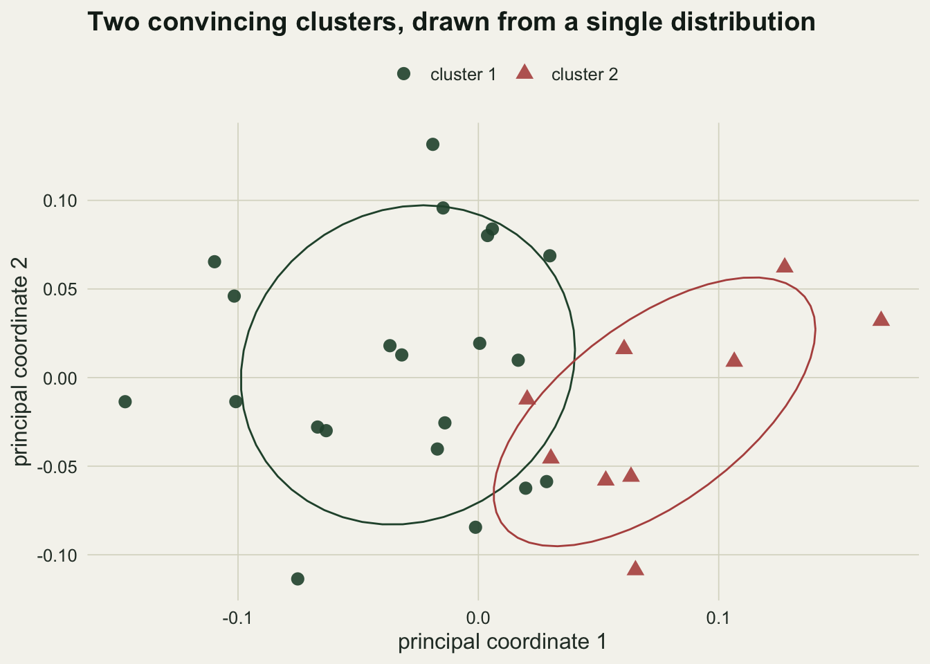

Figure 1: Principal coordinates ordination of thirty sites of pure Poisson noise, coloured by a two-group cut of the dendrogram computed from the same distances.

The statistic, in the open

The pseudo-F that PERMANOVA permutes can be written directly from the distance matrix, which makes the null easy to modify later.

pseudo_F <- function(d, g) {
  d2 <- as.matrix(d)^2
  n  <- length(g)
  ss_total  <- sum(d2[upper.tri(d2)]) / n
  ss_within <- 0
  for (lev in unique(g)) {
    idx <- which(g == lev)
    if (length(idx) < 2) next
    sub <- d2[idx, idx, drop = FALSE]
    ss_within <- ss_within + sum(sub[upper.tri(sub)]) / length(idx)
  }
  k <- length(unique(g))
  ((ss_total - ss_within) / (k - 1)) / (ss_within / (n - k))
}

f_hand <- pseudo_F(d1, g1)
f_gap  <- abs(f_hand - naive1_f)

The hand-written version returns 3.5981 against 3.5981 from adonis2, a difference of 8.0e-15.

How often does noise pass?

reps <- 200
linkages <- c("average", "complete", "ward.D2")
sweep <- data.frame(linkage = linkages, adonis = NA_real_, anosim = NA_real_,
                    mean_p = NA_real_, sd_p = NA_real_, smallest = NA_real_,
                    conditional = NA_real_, usable = NA_integer_)

for (i in seq_along(linkages)) {
  p_ad <- numeric(reps); p_an <- numeric(reps); small <- integer(reps)
  set.seed(20260805)
  for (r in seq_len(reps)) {
    d <- vegdist(noise_matrix())
    g <- cut_two(d, linkages[i])
    small[r] <- min(table(g))
    p_ad[r]  <- adonis2(d ~ factor(g), permutations = 199)$`Pr(>F)`[1]
    p_an[r]  <- anosim(d, factor(g), permutations = 199)$signif
  }
  sweep$adonis[i]      <- mean(p_ad <= 0.05) * 100
  sweep$anosim[i]      <- mean(p_an <= 0.05) * 100
  sweep$mean_p[i]      <- mean(p_ad)
  sweep$sd_p[i]        <- sd(p_ad)
  sweep$smallest[i]    <- median(small)
  sweep$conditional[i] <- mean(p_ad[small >= 2] <= 0.05) * 100
  sweep$usable[i]      <- sum(small >= 2)
}
sweep

   linkage adonis anosim   mean_p        sd_p smallest conditional usable
1  average   82.5   80.5 0.032425 0.026161354        1         100     73
2 complete   99.5   87.0 0.008050 0.009157884        9         100    187
3  ward.D2  100.0   93.5 0.005000 0.000000000       10         100    200

With Ward linkage, adonis2 declares the noise clusters significantly different in 100.0 per cent of 200 data sets, at a mean p-value of 0.0050 with a standard deviation of 0.0000. With 199 permutations the smallest attainable p-value is 0.005, so that mean is at the floor of the test.

ANOSIM is not a way out: it rejects in 93.5 per cent of the same data sets.

Why the published rates disagree

Rates quoted for this failure range from roughly eighty per cent to nearly one hundred. The linkage explains the spread, and it does so through the shape of the cut rather than through the test.

link_df <- rbind(
  data.frame(linkage = sweep$linkage, rate = sweep$adonis, subset = "all data sets"),
  data.frame(linkage = sweep$linkage, rate = sweep$conditional,
             subset = "cut gives two groups of 2 or more"))
link_df$linkage <- factor(link_df$linkage, levels = linkages)

ggplot(link_df, aes(x = linkage, y = rate, fill = subset)) +
  geom_col(position = position_dodge(width = 0.7), width = 0.6) +
  geom_text(aes(label = sprintf("%.1f", rate)),
            position = position_dodge(width = 0.7), vjust = -0.5,
            colour = te_body, size = 3.5) +
  scale_fill_manual(values = c("all data sets" = te_gold,
                               "cut gives two groups of 2 or more" = te_forest)) +
  scale_y_continuous(limits = c(0, 112)) +
  labs(x = NULL, y = "data sets declared significant (per cent)", fill = NULL,
       title = "The linkage decides the cut, and the cut decides the rate") +
  theme_datasheet() +
  theme(legend.position = "top")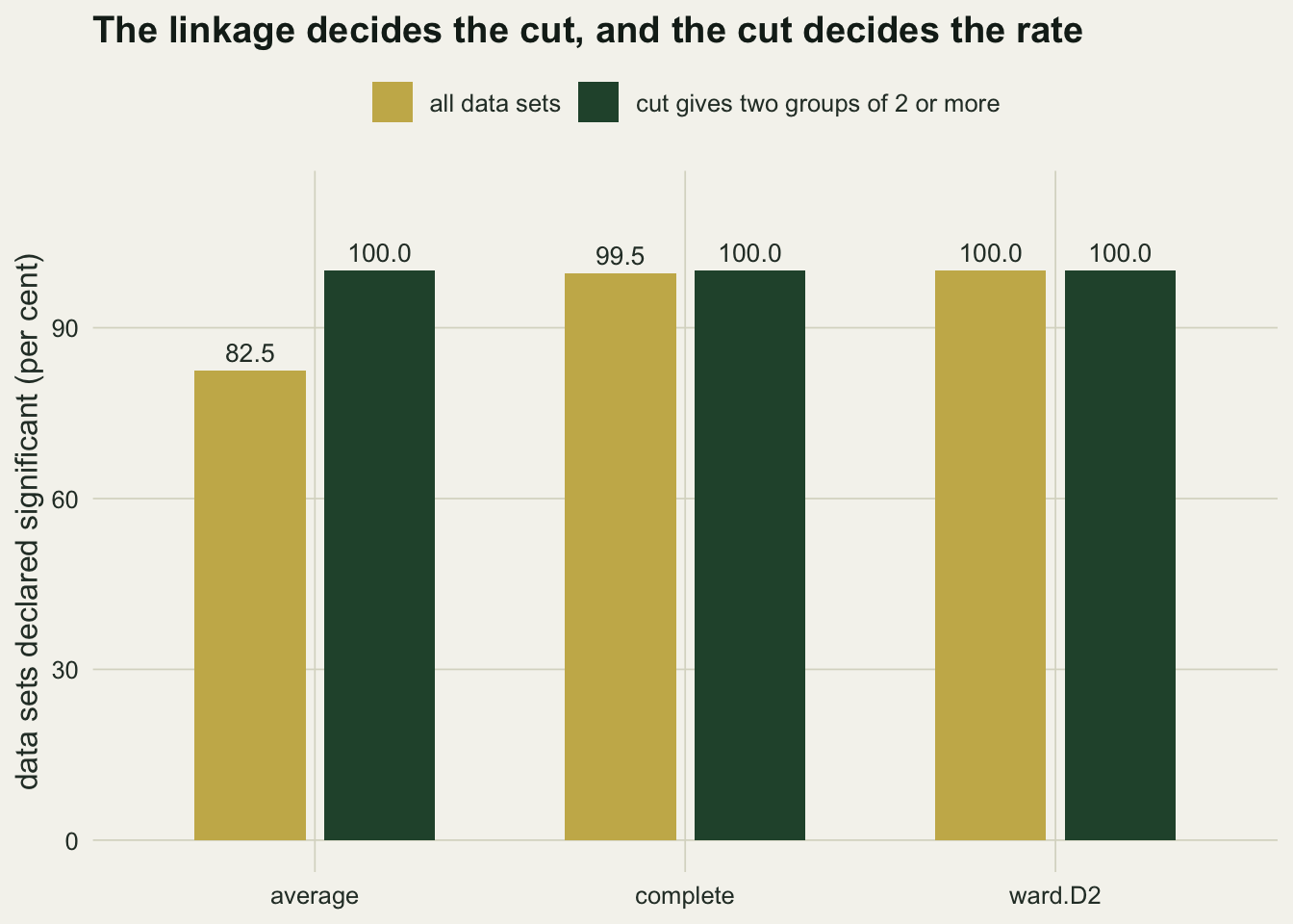

Figure 2: Rejection rate on unstructured data by linkage method, overall and restricted to data sets where the cut produced two clusters of at least two sites.

Average linkage on noisy Bray-Curtis distances tends to peel off one site at a time, so its median smaller cluster holds 1 site and the comparison is really an outlier test with almost nothing on one side of it. Ward linkage minimises within-group variance by construction, so it delivers balanced groups: median smaller cluster 10 sites.

The number that survives the difference is in the second set of bars. Restricted to data sets where the cut produced two groups of at least two sites, the rejection rate is 100 per cent for average linkage, 100 per cent for complete and 100 per cent for Ward. Whenever the dendrogram gives you two groups worth testing, the test on pure noise passes. The variation between reported rates is variation in how often the algorithm produces a degenerate cut, not variation in the size of the problem.

A null that includes the clustering

The defect is not in adonis2. It is that the null hypothesis being permuted is wrong: permuting group labels asks whether these labels are special, when the labels were chosen to be special. The honest null asks a different question, and it is the question the study means to ask: could a search of this kind, on data with no group structure, have produced a split this good?

To answer it, permute the raw data, run the entire pipeline again, and compare. Permuting within species columns destroys any association between sites while leaving each species with the abundance distribution it had.

corrected_p <- function(m, nperm = 199) {
  d <- vegdist(m)
  f_obs <- pseudo_F(d, cut_two(d))
  f_null <- replicate(nperm, {
    d_b <- vegdist(apply(m, 2, sample))
    pseudo_F(d_b, cut_two(d_b))
  })
  list(p = (1 + sum(f_null >= f_obs)) / (nperm + 1), f_obs = f_obs, f_null = f_null)
}

set.seed(4)
demo <- corrected_p(m1)
demo_p    <- demo$p
demo_fobs <- demo$f_obs
demo_fmed <- median(demo$f_null)

On the data set from the first figure, whose naive p-value was 0.005, the observed pseudo-F is 3.60 and the median pseudo-F from a reclustered permutation is 3.45. The corrected p-value is 0.410.

ggplot(data.frame(f = demo$f_null), aes(x = f)) +
  geom_histogram(bins = 24, fill = te_forest, colour = te_paper) +
  geom_vline(xintercept = demo_fobs, linetype = "dashed", colour = te_rust, linewidth = 0.9) +
  annotate("text", x = demo_fobs, y = Inf, vjust = 1.6, hjust = -0.05,
           colour = te_rust, size = 3.6, label = "observed") +
  labs(x = "pseudo-F from reclustered permutations", y = "permutations",
       title = "The comparison the naive test never makes") +
  theme_datasheet()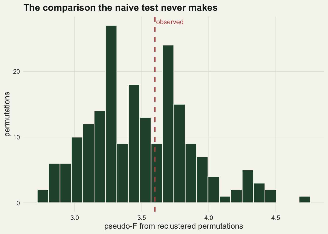

Figure 3: Null distribution of the pseudo-F statistic when the clustering is repeated inside every permutation, with the observed value marked.

Does the corrected test work?

A null that never rejects is not a test. It has to be calibrated on data without structure and able to find structure that is there.

set.seed(77)
n_null <- 100
p_corr_noise <- replicate(n_null, corrected_p(noise_matrix())$p)
corr_noise_rate <- mean(p_corr_noise <= 0.05) * 100
corr_se <- 100 * sqrt(0.05 * 0.95 / n_null)

structured_matrix <- function(sep) {
  half <- n_site / 2
  base <- exp(rnorm(n_sp, 1.5, 0.7))
  w <- rep(c(sep, 1 / sep), length.out = n_sp)
  rbind(matrix(rpois(half * n_sp, rep(base, each = half)), half, n_sp),
        matrix(rpois(half * n_sp, rep(base * w, each = half)), half, n_sp))
}

truth <- rep(1:2, each = n_site / 2)
n_str <- 30
run_structured <- function(sep, seed) {
  set.seed(seed)
  p_c <- numeric(n_str); rec <- numeric(n_str)
  for (r in seq_len(n_str)) {
    m <- structured_matrix(sep)
    g <- cut_two(vegdist(m))
    rec[r] <- max(mean(g == truth), mean(g != truth))
    p_c[r] <- corrected_p(m)$p
  }
  c(recovery = mean(rec) * 100, power = mean(p_c <= 0.05) * 100)
}
strong <- run_structured(1.8, 500)
weak   <- run_structured(1.25, 501)

On unstructured data the corrected test rejects in 9 per cent of 100 data sets, against a nominal five per cent with a Monte Carlo standard error of 2.2 percentage points. It is approximately calibrated rather than exact, and the reason is worth stating: shuffling within columns removes site-to-site variation in total abundance along with the group structure, so the null community is slightly tidier than the real one.

On data that does contain two groups, the cut recovers 98.8 per cent of the true labels when the groups are well separated, and the corrected test rejects in 100 per cent of runs. With a weaker separation the cut recovers 74.2 per cent of labels and the corrected test rejects in 47 per cent. It loses power as the structure fades, which is the behaviour a test is supposed to have.

summ <- data.frame(
  what = factor(c("naive, noise", "reclustered, noise",
                  "reclustered, strong groups", "reclustered, weak groups"),
                levels = c("naive, noise", "reclustered, noise",
                           "reclustered, strong groups", "reclustered, weak groups")),
  rate = c(sweep$adonis[sweep$linkage == "ward.D2"], corr_noise_rate,
           strong[["power"]], weak[["power"]]),
  kind = c("no structure in the data", "no structure in the data",
           "real groups", "real groups"))

ggplot(summ, aes(x = what, y = rate, fill = kind)) +
  geom_col(width = 0.55) +
  geom_hline(yintercept = 5, linetype = "dotted", colour = te_ink) +
  annotate("text", x = 0.62, y = 11, label = "nominal 5 per cent",
           hjust = 0, colour = te_ink, size = 3.3) +
  geom_text(aes(label = sprintf("%.0f", rate)), vjust = -0.5, colour = te_body, size = 4) +
  scale_fill_manual(values = c("no structure in the data" = te_rust,
                               "real groups" = te_forest)) +
  scale_y_continuous(limits = c(0, 112)) +
  labs(x = NULL, y = "runs declared significant (per cent)", fill = NULL,
       title = "What each test does when there is, and is not, something to find") +
  theme_datasheet() +
  theme(legend.position = "top", axis.text.x = element_text(angle = 15, hjust = 1))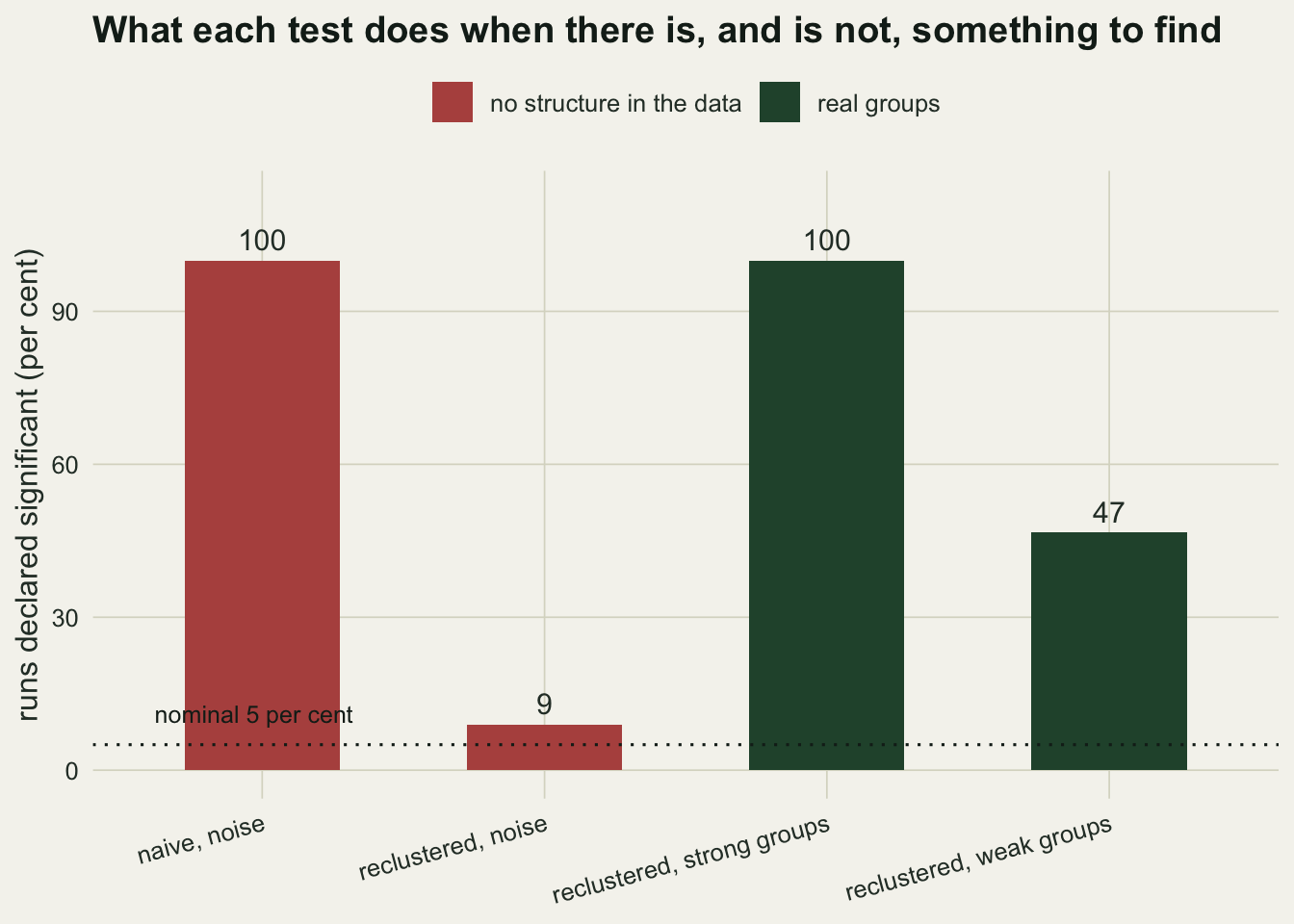

Figure 4: Rejection rates for the naive and the reclustered test, on unstructured data and on data with real groups.

What to report

If the groups came from the data, say so, and either run a null that repeats the search or drop the test. A classification can be useful without a p-value: describe how stable the cut is under resampling, how many sites change membership, and what the groups mean ecologically. The dendrogram tutorial covers the stability side; this post covers the inference side.

The rule generalises past clustering. Any grouping variable chosen by looking at the response, including an ordination axis split at a visual gap or a threshold picked from a scatter plot, carries the same defect, and the same repair: put the search inside the null.

Honest limits

The rates measured here belong to this generator, this matrix shape and this dissimilarity index. Thirty sites and twenty species with equal Poisson means is a maximally structureless case; a real survey has gradients, and a cut along a genuine gradient is not the same thing as a cut in noise, even when there are no discrete groups to find.

The reclustered null is approximate. Column-wise permutation is one choice of exchangeability, and it removes more than group structure. Where the design has a sampling structure of its own, that structure belongs in the permutation scheme, and the calibration should be checked again rather than assumed. Formal selective-inference tests for clustering exist and give exact control under stated assumptions, but they are built for specific distances and linkages, not for the Bray-Curtis and Ward combination used here.

References

Anderson MJ 2001 Austral Ecology 26(1):32-46 (10.1111/j.1442-9993.2001.01070.pp.x)

Clarke KR 1993 Australian Journal of Ecology 18(1):117-143 (10.1111/j.1442-9993.1993.tb00438.x)

Gao LL, Bien J, Witten D 2024 Journal of the American Statistical Association 119(545):332-342 (10.1080/01621459.2022.2116331)

Related tutorials

• Hierarchical clustering and dendrograms
• Common PERMANOVA mistakes
• Indicator species analysis
• Checking a clustering analysis