library(ggplot2)

te_pal <- list(forest = "#275139", green = "#2f8f63", sage = "#93a87f",
               clay = "#b5534e", gold = "#cda23f", line = "#dad9ca",
               ink = "#16241d", paper = "#f5f4ee")

theme_te <- function() {
  theme_minimal(base_size = 12) +
    theme(panel.grid.minor = element_blank(),
          panel.grid.major = element_line(colour = "#e7e6dc"),
          plot.background = element_rect(fill = "#f5f4ee", colour = NA),
          panel.background = element_rect(fill = "#f5f4ee", colour = NA),
          plot.title = element_text(face = "bold", colour = te_pal$ink),
          axis.title = element_text(colour = "#2c3a31"))
}Checking a genetic clustering analysis
R
population genetics
model diagnostics
ecology tutorial
ggplot2
Four checks for a genetic clustering analysis in R: unbalanced sampling, linked loci, variation between runs, and whether the structure survives a subsample.
A clustering run returns a barplot, and barplots are persuasive. The three tutorials before this one built the pieces: the ancestry model fitted by EM, the criteria that pick K, and assignment to a baseline of known populations. This one asks what would have to be true for the barplot to mean anything, and measures each condition on simulated data where the answer is known.
Four checks: sample the same populations unevenly, correlate the loci, restart the fit, and take away part of the data. Each one has a number attached, because “the clusters looked stable” is not a result.
The model is the usual one. Each individual i carries ancestry proportions q[i, ] over K sources, each source k has an allele frequency p[k, l] at every locus, and the expected frequency for that individual is the mixture of the two. A genotype counted as 0, 1 or 2 copies is then binomial with that frequency. The EM step below writes the whole update as four matrix products, which is what keeps 40 refits affordable.
sim_sources <- function(n_loci, n_k, sigma, block, seed) {
  set.seed(seed)
  p_anc <- runif(n_loci, 0.2, 0.8)
  n_block <- ceiling(n_loci / block)
  dev <- matrix(rnorm(n_k * n_block), n_k, n_block)
  dev <- dev[, rep(seq_len(n_block), each = block)[seq_len(n_loci)],
             drop = FALSE]
  pp <- plogis(qlogis(rep(p_anc, each = n_k)) + sigma * as.vector(dev))
  pmin(pmax(matrix(pp, n_k, n_loci), 0.02), 0.98)
}

locus_fst <- function(p_src) {
  p_bar <- colMeans(p_src)
  (colMeans(p_src^2) - p_bar^2) / (p_bar * (1 - p_bar))
}

draw_geno <- function(p_src, n_per) {
  grp <- rep(seq_len(nrow(p_src)), times = n_per)
  pm <- p_src[grp, , drop = FALSE]
  list(geno = matrix(rbinom(length(pm), 2, as.vector(pm)), nrow = nrow(pm)),
       grp = grp)
}

em_fit <- function(geno, n_k, seed, n_iter = 300) {
  set.seed(seed)
  q_mat <- matrix(runif(nrow(geno) * n_k, 0.2, 0.8), nrow(geno), n_k)
  q_mat <- q_mat / rowSums(q_mat)
  p_mat <- matrix(runif(n_k * ncol(geno), 0.1, 0.9), n_k, ncol(geno))
  eps <- 1e-6
  clamp <- function(m) pmin(pmax(m, eps), 1 - eps)
  g2 <- 2 - geno
  for (it in seq_len(n_iter)) {
    fr <- clamp(q_mat %*% p_mat)
    aa <- geno / fr
    bb <- g2 / (1 - fr)
    q_num <- q_mat * (aa %*% t(p_mat) + bb %*% t(1 - p_mat))
    p_num <- p_mat * t(crossprod(aa, q_mat))
    p_den <- p_num + (1 - p_mat) * t(crossprod(bb, q_mat))
    q_mat <- q_num / rowSums(q_num)
    p_mat <- clamp(p_num / pmax(p_den, eps))
  }
  fr <- clamp(q_mat %*% p_mat)
  list(q = q_mat, loglik = sum(geno * log(fr) + g2 * log(1 - fr)))
}

multi_fit <- function(geno, n_k, n_start, seed, n_iter = 300) {
  set.seed(seed)
  sds <- sample(1e6, n_start)
  lapply(sds, function(s) em_fit(geno, n_k, s, n_iter))
}

best_fit <- function(geno, n_k, n_start, seed, n_iter = 300) {
  runs <- multi_fit(geno, n_k, n_start, seed, n_iter)
  runs[[which.max(sapply(runs, function(z) z$loglik))]]
}
Two clusters carry no labels, so nothing can be compared until the labels are matched. With K small the exact solution is to try every permutation of the columns and keep the one that agrees best, which is the full search that CLUMPP does; larger K needs the Hungarian algorithm instead. Agreement is reported as one minus the mean absolute difference between the two ancestry matrices, so 1 is identity.
perm_list <- function(n_k) {
  if (n_k == 1) return(matrix(1L))
  out <- NULL
  sm <- perm_list(n_k - 1)
  for (i in seq_len(n_k)) {
    rest <- setdiff(seq_len(n_k), i)
    out <- rbind(out, cbind(i, matrix(rest[sm], nrow(sm))))
  }
  out
}

align_q <- function(q_ref, q_new) {
  pp <- perm_list(ncol(q_ref))
  sc <- apply(pp, 1, function(o) mean(abs(q_ref - q_new[, o, drop = FALSE])))
  w <- which.min(sc)
  list(q = q_new[, pp[w, ], drop = FALSE], agree = 1 - sc[w])
}

true_q <- function(grp, n_k) {
  out <- matrix(0, length(grp), n_k)
  out[cbind(seq_along(grp), grp)] <- 1
  out
}

group_error <- function(fit_q, grp, n_k) {
  qt <- true_q(grp, n_k)
  al <- align_q(qt, fit_q)
  list(mae = tapply(seq_along(grp), grp,
                    function(i) mean(abs(qt[i, ] - al$q[i, , drop = FALSE]))),
       self = tapply(seq_along(grp), grp,
                     function(i) mean(al$q[cbind(i, grp[i])])),
       q = al$q)
}
Check 1: are the clusters the populations or the sample sizes?
Three source populations, drawn from one ancestral frequency spectrum with the same amount of drift applied to each, so their differentiation is genuinely equal. Sample them the way a field project usually does: 100 individuals from the accessible population, 30 from the awkward one, 10 from the remote one. Then fit at the true K = 3 and compare with a balanced sample of the same total size.
n_loci <- 80
sigma_src <- 0.68
n_uneven <- c(100, 30, 10)
n_balanced <- c(47, 47, 46)

p_src <- sim_sources(n_loci, 3, sigma_src, 1, 71001)
cat("loci:", n_loci, " individuals in each design:", sum(n_uneven),
    " mean per-locus Fst among the three sources:",
    round(mean(locus_fst(p_src)), 4), "\n")
loci: 80 individuals in each design: 140 mean per-locus Fst among the three sources: 0.064 set.seed(71002)
dat_un <- draw_geno(p_src, n_uneven)
set.seed(71003)
dat_ba <- draw_geno(p_src, n_balanced)
fit_un <- best_fit(dat_un$geno, 3, 3, 71004)
fit_ba <- best_fit(dat_ba$geno, 3, 3, 71005)
err_un <- group_error(fit_un$q, dat_un$grp, 3)
err_ba <- group_error(fit_ba$q, dat_ba$grp, 3)
set.seed(71006)
keep_un <- unlist(lapply(1:3, function(k) {
idx <- which(dat_un$grp == k)
if (length(idx) > 10) sample(idx, 10) else idx
}))
fit_sub <- best_fit(dat_un$geno[keep_un, ], 3, 3, 71007)
err_sub <- group_error(fit_sub$q, dat_un$grp[keep_un], 3)
design_lab <- c("uneven 100/30/10", "balanced 47/47/46",
"subsampled 10/10/10")
tab_design <- data.frame(
design = rep(design_lab, each = 3),
source = rep(c("A", "B", "C"), 3),
sampled = c(n_uneven, n_balanced, rep(10, 3)),
mean_self_q = round(c(err_un$self, err_ba$self, err_sub$self), 3),
mae_q = round(c(err_un$mae, err_ba$mae, err_sub$mae), 3))
print(tab_design, row.names = FALSE) design source sampled mean_self_q mae_q
uneven 100/30/10 A 100 0.563 0.291
uneven 100/30/10 B 30 0.740 0.173
uneven 100/30/10 C 10 0.515 0.323
balanced 47/47/46 A 47 0.721 0.186
balanced 47/47/46 B 47 0.655 0.230
balanced 47/47/46 C 46 0.772 0.152
subsampled 10/10/10 A 10 0.759 0.160
subsampled 10/10/10 B 10 0.703 0.198
subsampled 10/10/10 C 10 0.733 0.178Read the mean_self_q column against the balanced rows rather than against 1. With 80 loci and a mean per-locus Fst of 0.064 the model cannot pin an unadmixed individual to one source, so even the balanced design reports substantial mixed ancestry, and that is the baseline.
Against that baseline the uneven design comes out worse, and this table says where the loss lands. Source C, the one with 10 individuals, gets a mean self-ancestry of 0.515 against the 0.772 of the balanced rows, and source A, the one with 100, drops to 0.563 from 0.721. On this dataset the middle group is the only one that does not lose ground. Only one of the two damaged clusters still corresponds to a single source: the large sample has been divided between two clusters, and the remote population shares one of them rather than holding its own.
One dataset is an anecdote, so repeat the whole thing.
n_rep <- 16
rep_rows <- NULL
for (r in seq_len(n_rep)) {
  ps <- sim_sources(n_loci, 3, sigma_src, 1, 71100 + r)
  set.seed(71200 + r)
  dd_un <- draw_geno(ps, n_uneven)
  set.seed(71300 + r)
  dd_ba <- draw_geno(ps, n_balanced)
  set.seed(71400 + r)
  kk <- unlist(lapply(1:3, function(k) {
    idx <- which(dd_un$grp == k)
    if (length(idx) > 10) sample(idx, 10) else idx
  }))
  fits <- list(group_error(best_fit(dd_un$geno, 3, 2, 71500 + r)$q,
                           dd_un$grp, 3),
               group_error(best_fit(dd_ba$geno, 3, 2, 71600 + r)$q,
                           dd_ba$grp, 3),
               group_error(best_fit(dd_un$geno[kk, ], 3, 2, 71700 + r)$q,
                           dd_un$grp[kk], 3))
  for (d in 1:3) {
    rep_rows <- rbind(rep_rows, data.frame(
      sim = r, design = design_lab[d], source = c("A", "B", "C"),
      self = as.numeric(fits[[d]]$self), mae = as.numeric(fits[[d]]$mae)))
  }
}

tab_rep <- aggregate(cbind(self, mae) ~ design + source, rep_rows, mean)
tab_rep$no_own_cluster <- aggregate(self ~ design + source, rep_rows,
                                    function(z) mean(z < 0.5))$self
tab_rep <- tab_rep[order(match(tab_rep$design, design_lab), tab_rep$source), ]
tab_rep$self <- round(tab_rep$self, 3)
tab_rep$mae <- round(tab_rep$mae, 3)
tab_rep$no_own_cluster <- round(tab_rep$no_own_cluster, 3)
cat("replicate simulations:", n_rep, " starts per fit: 2\n")
replicate simulations: 16 starts per fit: 2print(tab_rep, row.names = FALSE) design source self mae no_own_cluster
uneven 100/30/10 A 0.578 0.281 0.062
uneven 100/30/10 B 0.683 0.211 0.000
uneven 100/30/10 C 0.595 0.270 0.125
balanced 47/47/46 A 0.712 0.192 0.000
balanced 47/47/46 B 0.695 0.203 0.000
balanced 47/47/46 C 0.707 0.195 0.000
subsampled 10/10/10 A 0.691 0.206 0.062
subsampled 10/10/10 B 0.727 0.182 0.000
subsampled 10/10/10 C 0.697 0.202 0.062by_design <- split(rep_rows, match(rep_rows$design, design_lab))
cat("replicates out of", n_rep,
"with a larger error than the balanced design, uneven:",
tapply(by_design[[1]]$mae > by_design[[2]]$mae,
by_design[[1]]$source, sum),
" subsampled:",
tapply(by_design[[3]]$mae > by_design[[2]]$mae,
by_design[[3]]$source, sum), "\n")replicates out of 16 with a larger error than the balanced design, uneven: 16 7 11 subsampled: 9 5 6 Sixteen independent simulations, each with fresh source frequencies and fresh genotypes. Averaged over them, the mean absolute error in q for the small population is 0.270 under uneven sampling against 0.195 under balanced sampling, and for the large population 0.281 against 0.192. The no_own_cluster column counts how often a group failed to hold a cluster of its own, defined as a mean self-ancestry below 0.5: never in the balanced design, at a rate of 0.125 for the small population and 0.062 for the large one when the sampling was uneven.
The paired count in the last line is the sharper statement, because it compares the two designs on the same simulated populations rather than on averages. The uneven design gave the larger error in all 16 replicates for source A and in 11 of 16 for source C, against 7 of 16 for the middle group, which is what no effect looks like.
The fix is cheap and it works. Refitting on 10 individuals per group, which discards most of the data, recovers the structure better than the full uneven sample: mean absolute errors of 0.206, 0.182 and 0.202 across the three sources, against 0.281, 0.211 and 0.270. That is level with the balanced design, which managed 0.192, 0.203 and 0.195, and the paired counts say the same thing: the subsampled fit lost to the balanced fit in 9, 5 and 6 replicates out of 16, so the two are hard to tell apart. Subsampling does not remove the failures, losing a cluster at a rate of 0.062 for two of the three sources. Information was not the problem, though. Balance was.
bar_df <- NULL
short_lab <- c("uneven", "balanced", "subsampled")
for (d in 1:3) {
  qq <- list(err_un$q, err_ba$q, err_sub$q)[[d]]
  gg <- list(dat_un$grp, dat_ba$grp, dat_un$grp[keep_un])[[d]]
  for (k in 1:3) {
    bar_df <- rbind(bar_df, data.frame(
      design = short_lab[d], source = paste("source", c("A", "B", "C"))[gg],
      ind = ave(seq_along(gg), gg, FUN = seq_along),
      n_grp = ave(seq_along(gg), gg, FUN = length),
      cluster = paste("cluster", k), q = qq[, k]))
  }
}
bar_df$design <- factor(bar_df$design, levels = short_lab)
bar_df$pos <- (bar_df$ind - 0.5) / bar_df$n_grp

ggplot(bar_df, aes(pos, q, fill = cluster, width = 1 / n_grp)) +
  geom_col() +
  facet_grid(design ~ source) +
  scale_fill_manual(values = c(te_pal$forest, te_pal$gold, te_pal$clay),
                    name = NULL) +
  scale_y_continuous(expand = c(0, 0)) +
  scale_x_continuous(expand = c(0, 0)) +
  labs(title = "Unequal samples move the cluster boundaries",
       subtitle = "one set of source populations, 80 loci, sampled 100/30/10 then 47/47/46 then 10/10/10",
       x = "individual, ordered within source", y = "ancestry proportion") +
  theme_te() +
  theme(legend.position = "bottom", panel.grid = element_blank(),
        axis.text.x = element_blank(),
        strip.text.y = element_text(angle = 0))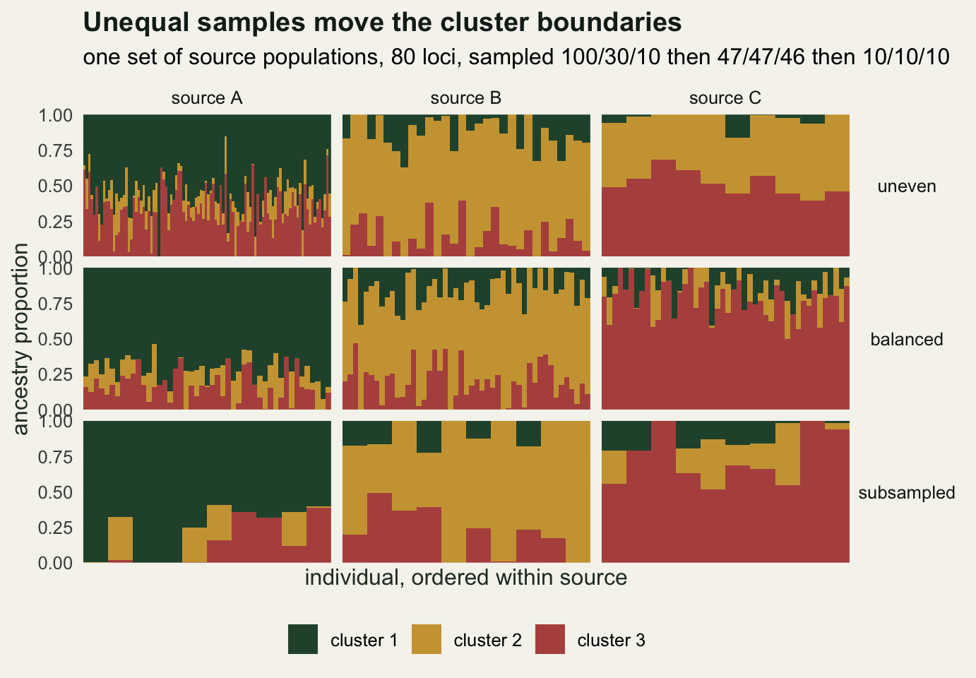
Check 2: how many independent loci are there?
Every clustering program treats loci as independent, which is how a marker panel of a few hundred single nucleotide polymorphisms turns into a log-likelihood with hundreds of terms. Markers on the same chromosome are not independent, and neither are markers that respond to the same demographic accident. Simulate that directly: build the source frequencies in blocks of 10 loci that share one frequency deviation, so 200 nominal loci carry 20 independent signals, and give the model no hint.
The effective number of independent loci is measurable without fitting anything. Take a statistic that averages over loci, here the mean per-locus Fst among the three sources, and compare its variance across replicate simulations with the variance among loci within one simulation. The ratio is the number of independent loci the average behaves like.
n_nominal <- 200
block_size <- 10
design_loci <- c("200 independent loci", "200 loci in blocks of 10",
                 "20 independent loci")
n_sim <- 400
eff_tab <- NULL
for (dn in seq_along(design_loci)) {
  nl <- if (dn == 3) 20 else n_nominal
  bl <- if (dn == 2) block_size else 1
  within_var <- numeric(n_sim)
  sim_means <- numeric(n_sim)
  for (r in seq_len(n_sim)) {
    fv <- locus_fst(sim_sources(nl, 3, sigma_src, bl, 72000 + 1000 * dn + r))
    within_var[r] <- var(fv)
    sim_means[r] <- mean(fv)
  }
  eff_tab <- rbind(eff_tab, data.frame(
    design = design_loci[dn], nominal_loci = nl,
    mean_fst = round(mean(sim_means), 4),
    effective_loci = round(mean(within_var) / var(sim_means), 1)))
}
cat("replicate simulations per design:", n_sim, "\n")
replicate simulations per design: 400 print(eff_tab, row.names = FALSE) design nominal_loci mean_fst effective_loci
200 independent loci 200 0.0589 204.1
200 loci in blocks of 10 200 0.0594 21.8
20 independent loci 20 0.0589 19.8The estimator recovers the truth where the truth is known: 204.1 for the panel of 200 independent loci and 19.8 for the panel of 20. The blocked panel has 200 loci and behaves like 21.8 of them, and its mean per-locus Fst, 0.0594, matches the other two designs, so nothing about the differentiation has changed. Now fit all three panels over a range of K and look at what the log-likelihood does.
ll_tab <- NULL
for (dn in seq_along(design_loci)) {
  nl <- if (dn == 3) 20 else n_nominal
  bl <- if (dn == 2) block_size else 1
  ps <- sim_sources(nl, 3, sigma_src, bl, 72500 + dn)
  set.seed(72600 + dn)
  dd <- draw_geno(ps, n_balanced)
  for (kk in 1:4) {
    runs <- multi_fit(dd$geno, kk, 3, 72700 + 10 * dn + kk)
    lls <- sapply(runs, function(z) z$loglik)
    bb <- runs[[which.max(lls)]]
    ll_tab <- rbind(ll_tab, data.frame(
      design = design_loci[dn], K = kk, loglik = round(max(lls), 1),
      start_spread = round(max(lls) - min(lls), 2),
      mae_q = if (kk == 3) round(mean(group_error(bb$q, dd$grp, 3)$mae), 3)
              else NA_real_))
  }
}
for (dn in design_loci) {
  ii <- ll_tab$design == dn
  ll_tab$step_gain[ii] <- round(c(NA, diff(ll_tab$loglik[ii])), 1)
}
print(ll_tab, row.names = FALSE)
design K loglik start_spread mae_q step_gain
200 independent loci 1 -34994.7 0.00 NA NA
200 independent loci 2 -33960.7 1.21 NA 1034.0
200 independent loci 3 -32926.6 4.93 0.159 1034.1
200 independent loci 4 -32657.8 27.90 NA 268.8
200 loci in blocks of 10 1 -34978.4 0.00 NA NA
200 loci in blocks of 10 2 -33964.0 1.23 NA 1014.4
200 loci in blocks of 10 3 -33328.2 17.89 0.202 635.8
200 loci in blocks of 10 4 -33068.7 42.83 NA 259.5
20 independent loci 1 -3637.6 0.00 NA NA
20 independent loci 2 -3443.0 0.82 NA 194.6
20 independent loci 3 -3307.1 14.21 0.278 135.9
20 independent loci 4 -3198.6 13.82 NA 108.5Compare the blocked panel with the 20 independent loci it is worth. Going from K = 2 to K = 3, the true number, the blocked panel gains 635.8 in log-likelihood and the 20 independent loci gain 135.9: roughly five times as much, from two datasets carrying the same information about how many sources exist. Any criterion built on differences of log-likelihood, and that includes every information criterion, reads the nominal locus count.
The run-to-run spread does not follow the gain, and that gives the game away. At K = 3 the three starts on the 200 independent loci land within 4.93 of each other; the blocked panel spreads over 17.89 and the 20 independent loci over 14.21. So on this run the blocked panel produces a large, confident-looking log-likelihood gain from a likelihood surface no better settled than the small panel’s. A spread taken from three starts is itself noisy, so the reading is that the extra 180 nominal loci buy no extra stability, not that the blocked panel is reliably the least settled of the three.
Parameter recovery stays closer to the independent panel than to the 20 loci, and it is worth saying why. The mean absolute error in q at K = 3 is 0.159 for the independent panel, 0.202 for the blocked one and 0.278 for the 20 loci. Blocked loci beat 20 loci here because each of the 200 genotypes is still an independent binomial draw, so the sampling noise in an individual’s genotypes does average down. What does not average down is the evidence about which sources exist, and that is what the choice of K depends on.
gain_df <- subset(ll_tab, K > 1)
gain_df$design <- factor(gain_df$design, levels = design_loci)

ggplot(gain_df, aes(K, step_gain, colour = design, shape = design)) +
  geom_line(linewidth = 0.9) +
  geom_point(size = 3) +
  scale_x_continuous(breaks = 2:4) +
  scale_y_log10() +
  scale_colour_manual(values = c(te_pal$forest, te_pal$clay, te_pal$gold),
                      name = NULL) +
  scale_shape_manual(values = c(16, 17, 15), name = NULL) +
  labs(title = "Linked loci inflate the gain, not the information",
       subtitle = "log-likelihood gained from K - 1 to K, best of three starts",
       x = "number of clusters K",
       y = "log-likelihood gain (log scale)") +
  theme_te() +
  theme(legend.position = "bottom")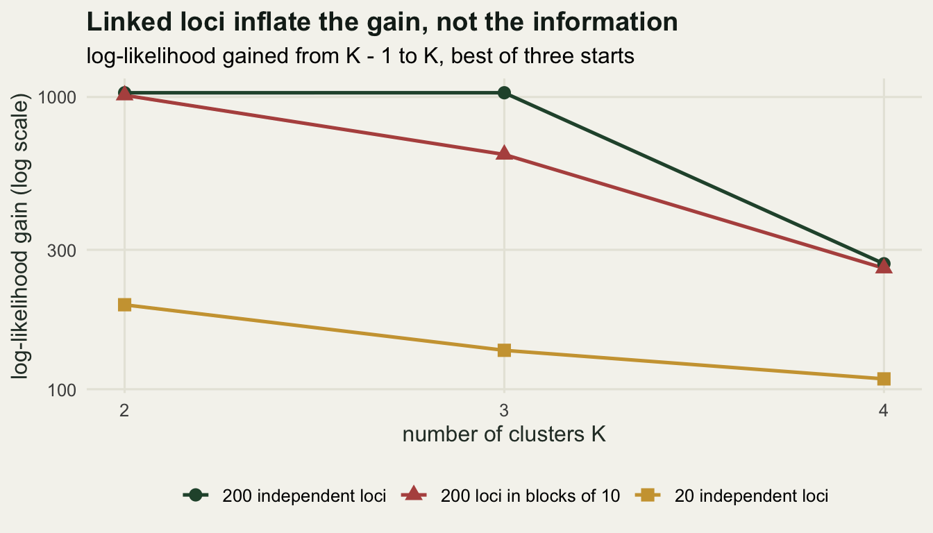
Check 3: how much does the answer move between runs?
The likelihood surface of this model is not concave and the EM step is a hill climb, so a run reports the top of whichever hill it started on. Take the uneven dataset from check 1, keep everything else fixed, and restart the fit 40 times from random values. This check gets a longer budget of 600 iterations per run, so that what remains is the difference between hills rather than between unfinished climbs.
n_start <- 40
long_iter <- 600
runs_ms <- multi_fit(dat_un$geno, 3, n_start, 73001, long_iter)
ll_ms <- sapply(runs_ms, function(z) z$loglik)

agree_mat <- matrix(1, n_start, n_start)
for (i in seq_len(n_start - 1)) {
  for (j in (i + 1):n_start) {
    ag <- align_q(runs_ms[[i]]$q, runs_ms[[j]]$q)$agree
    agree_mat[i, j] <- ag
    agree_mat[j, i] <- ag
  }
}

solution_groups <- function(am, lls, thr) {
  lab <- rep(NA_integer_, length(lls))
  nxt <- 0
  for (i in order(lls, decreasing = TRUE)) {
    if (is.na(lab[i])) {
      nxt <- nxt + 1
      lab[is.na(lab) & am[i, ] > thr] <- nxt
    }
  }
  lab
}
lab_ms <- solution_groups(agree_mat, ll_ms, 0.90)

set.seed(73002)
q_best <- runs_ms[[which.max(ll_ms)]]$q
floor_agree <- mean(replicate(20, align_q(q_best,
                                          q_best[sample(nrow(q_best)), ])$agree))

cat("random starts:", n_start, " EM iterations per start:", long_iter, "\n")
random starts: 40 EM iterations per start: 600 cat("log-likelihood best:", round(max(ll_ms), 1),
" worst:", round(min(ll_ms), 1),
" spread:", round(max(ll_ms) - min(ll_ms), 1),
" sd:", round(sd(ll_ms), 2), "\n")log-likelihood best: -13081.9 worst: -13110.3 spread: 28.4 sd: 8.72 cat("starts within 1 unit of the best:", sum(ll_ms > max(ll_ms) - 1), "\n")starts within 1 unit of the best: 6 cat("solution groups at 0.10 tolerance:", max(lab_ms),
" sizes:", sort(as.integer(table(lab_ms)), decreasing = TRUE), "\n")solution groups at 0.10 tolerance: 5 sizes: 21 15 2 1 1 cat("solution groups at 0.05 tolerance:",
max(solution_groups(agree_mat, ll_ms, 0.95)), "\n")solution groups at 0.05 tolerance: 14 cat("mean pairwise agreement:",
round(mean(agree_mat[upper.tri(agree_mat)]), 4),
" lowest pair:", round(min(agree_mat), 4),
" chance level:", round(floor_agree, 4), "\n")mean pairwise agreement: 0.882 lowest pair: 0.7754 chance level: 0.7366 Forty starts, one dataset, one value of K, and the log-likelihood ranges over 28.4 units. Six of the 40 reach within one unit of the best. Grouping the runs by their aligned ancestry matrices, with two runs counted as the same solution when their mean absolute difference is below 0.10, gives 5 groups, of which the two largest hold 21 and 15 runs. Tightening the tolerance to 0.05 gives 14, which is a reminder that the count is a property of the tolerance and not of nature; the finding is that a few solutions absorb most of the 40 starts.
The mean pairwise agreement is 0.882 against a chance level of 0.7366, that last figure obtained by shuffling the individuals of the best solution and re-aligning. So the runs agree with each other far more than random matrices do, and still disagree about roughly one ancestry unit in ten.
What follows for a paper is the same argument as selection frequency in conservation prioritisation, where one optimal reserve network says much less than the proportion of solutions that keep a site. The honest output of a clustering analysis is the distribution over runs: how many distinct solutions appeared, how many starts found each, and which individuals move between them. A single barplot is one draw from that distribution, chosen because it had the best log-likelihood among draws that were 28.4 units apart.
ord_ms <- order(ll_ms, decreasing = TRUE)
heat_df <- data.frame(
  row = rep(seq_len(n_start), times = n_start),
  col = rep(seq_len(n_start), each = n_start),
  agreement = as.vector(agree_mat[ord_ms, ord_ms]))

ggplot(heat_df, aes(row, col, fill = agreement)) +
  geom_raster() +
  coord_equal() +
  scale_fill_gradient(low = te_pal$paper, high = te_pal$forest,
                      name = "agreement") +
  labs(title = "Two solutions, forty starts",
       subtitle = "mean agreement 0.882, chance level 0.7366",
       x = "run, ranked by log-likelihood",
       y = "run, ranked by log-likelihood") +
  theme_te() +
  theme(panel.grid = element_blank())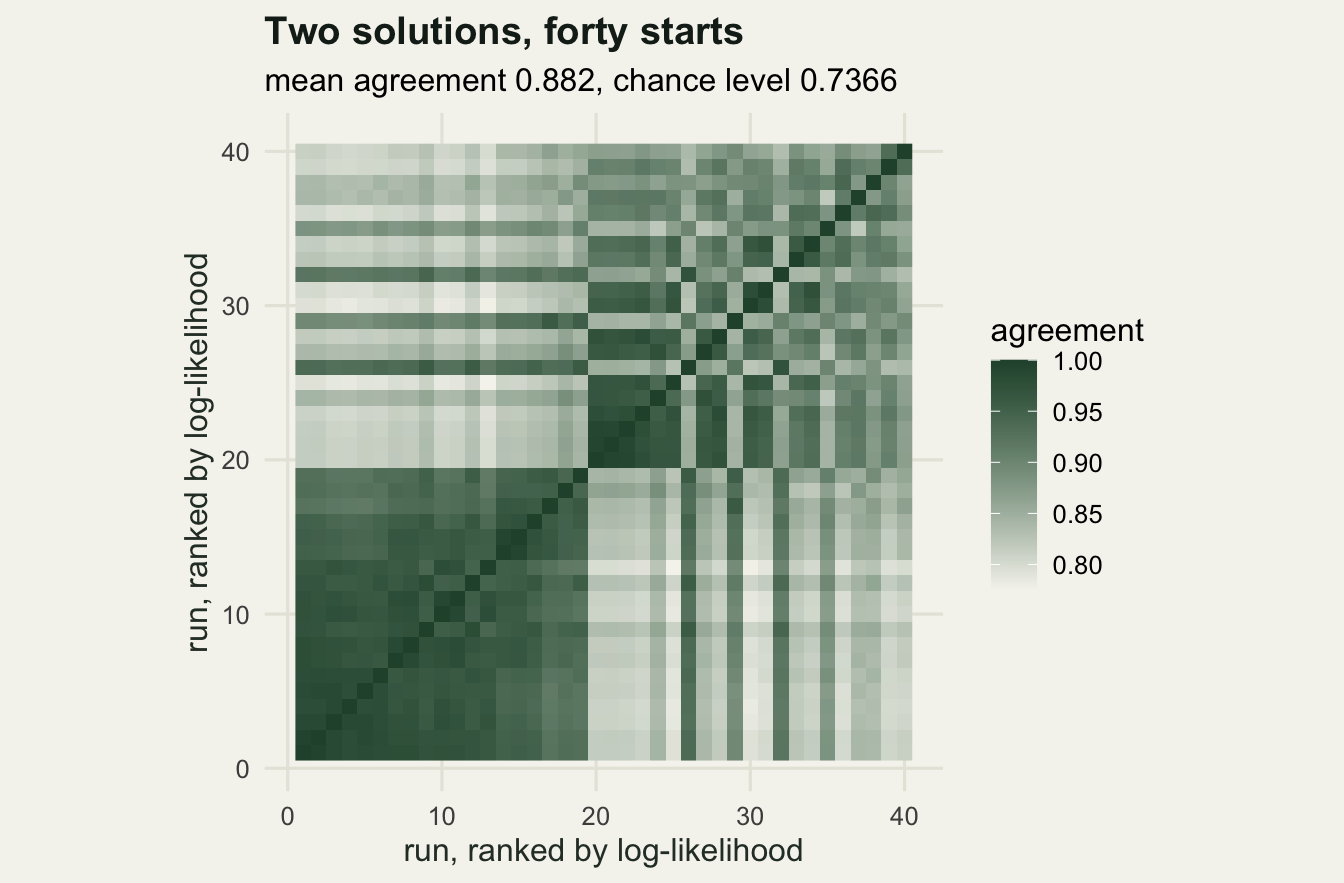
Check 4: does the structure survive a subsample?
Two resampling checks, both with a number at the end. First drop loci: refit on a random fraction of the 80 loci, several draws each, and measure agreement with the full-data fit on the balanced dataset. This is the closest thing the analysis has to an internal precision estimate.
frac_grid <- c(0.1, 0.25, 0.5, 0.75)
n_draw <- 4
sub_tab <- NULL
set.seed(74001)
for (fr in frac_grid) {
  ags <- numeric(n_draw)
  for (d in seq_len(n_draw)) {
    sel <- sample(n_loci, round(fr * n_loci))
    ff <- best_fit(dat_ba$geno[, sel], 3, 2,
                   74100 + 100 * d + round(100 * fr))
    ags[d] <- align_q(fit_ba$q, ff$q)$agree
  }
  sub_tab <- rbind(sub_tab, data.frame(
    fraction = fr, loci = round(fr * n_loci),
    mean_agreement = round(mean(ags), 4), lowest = round(min(ags), 4)))
}
cat("draws per fraction:", n_draw, "\n")
draws per fraction: 4 print(sub_tab, row.names = FALSE) fraction loci mean_agreement lowest
0.10 8 0.7723 0.7635
0.25 20 0.8382 0.8145
0.50 40 0.9062 0.8885
0.75 60 0.9354 0.9158Half the loci reproduce the full-data ancestry matrix at 0.9062, three quarters at 0.9354. A tenth of them, 8 loci, gives 0.7723, which against the chance level of 0.7366 from check 3 is barely a result at all. The reading for a real panel is that this curve should be flat near the full data: if halving the markers moves the ancestry proportions appreciably, the reported proportions are a property of the panel.
frac_df <- data.frame(fraction = c(sub_tab$fraction, 1),
                      agreement = c(sub_tab$mean_agreement, 1),
                      lowest = c(sub_tab$lowest, 1))

ggplot(frac_df, aes(fraction, agreement)) +
  geom_hline(yintercept = floor_agree, linetype = "dashed",
             colour = te_pal$clay) +
  geom_hline(yintercept = 1, colour = te_pal$line) +
  geom_linerange(aes(ymin = lowest, ymax = agreement),
                 colour = te_pal$sage, linewidth = 1.1) +
  geom_line(colour = te_pal$forest, linewidth = 0.9) +
  geom_point(colour = te_pal$forest, size = 2.6) +
  annotate("text", x = 0.34, y = floor_agree + 0.008,
           label = "chance level", colour = te_pal$clay, size = 3.4) +
  labs(title = "Half the markers is not the same answer",
       subtitle = "agreement with the full-data fit, balanced sample of 140 individuals",
       x = "fraction of the 80 loci retained",
       y = "agreement with the full-data fit") +
  theme_te()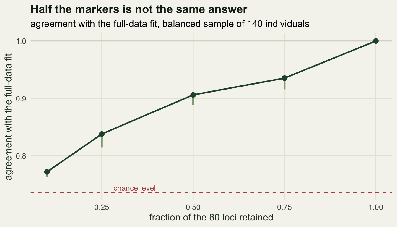
The second check is harder on the model. Drop source C from the dataset entirely, as an unvisited population would be, and refit at K = 2.
keep_ab <- which(dat_ba$grp != 3)
fit_drop <- best_fit(dat_ba$geno[keep_ab, ], 2, 3, 75001)
q_three <- align_q(true_q(dat_ba$grp, 3), fit_ba$q)$q
q_two <- align_q(true_q(dat_ba$grp[keep_ab], 2), fit_drop$q)$q
before <- t(sapply(1:2, function(k) colMeans(q_three[dat_ba$grp == k, ])))
after <- t(sapply(1:2, function(k)
  colMeans(q_two[dat_ba$grp[keep_ab] == k, , drop = FALSE])))

print(data.frame(source = c("A", "B"),
                 own_q_with_C = round(diag(before), 3),
                 q_on_C_cluster = round(before[, 3], 3),
                 own_q_without_C = round(diag(after), 3)),
      row.names = FALSE)
source own_q_with_C q_on_C_cluster own_q_without_C
A 0.721 0.160 0.860
B 0.655 0.193 0.795Nobody in sources A and B changed genotype, and their ancestry proportions changed anyway. Source A went from a mean self-ancestry of 0.721 to 0.86, source B from 0.655 to 0.795, and most of the 0.16 and 0.193 they had been assigning to the C cluster went back to their own. That is not an error in either fit. It is what q means: a proportion relative to the set of sources the model was given, not a fraction of an individual’s history. Two studies on the same species that sampled different populations will report different ancestry proportions for the same individual, and both can be right.
The honest limit
The four checks constrain a clustering analysis; they do not validate it. Between them they say whether the design decides the clusters, how much evidence the loci actually carry, how much of the answer is the random seed, and how much survives losing data. All four are internal, and all four can pass on an analysis whose conclusion is wrong.
Two failure modes survive every one of them. The first is continuous variation. A species distributed along a gradient of gene flow has no clusters at all, and this model has no way of saying so: it returns clusters because clusters are all it can return, the criteria for K behave much as they do on real clusters, and the previous tutorial measured that. No internal diagnostic sees it, because the fit is not failing.
The second is the population nobody sampled. Check 4 makes the point from the inside: removing a source changed the ancestry proportions of everyone else, and nothing in the reduced fit flagged that a source was missing. Run the same argument forwards and a study that never visited a source population gets a self-consistent, reproducible, well-supported answer to a question about a different set of sources. That failure cannot be detected from genotypes at all, at any sample size.
So the outputs worth reporting are narrower than a barplot. A distribution over runs rather than one run. A map of where the clusters sit, because a cluster that is not geographically coherent is usually a sampling artefact. And a plain statement of what was sampled and what was not, since that is the assumption the ancestry proportions are relative to.
Where to go next
This closes the clustering cluster. The wider population genetics checking tutorial covers the ground underneath it: how many loci and individuals a usable Fst needs, how to tell a marker problem from a biological one, and why an outlier test for selection needs a demographic null first.
References
Puechmaille SJ 2016 Molecular Ecology Resources 16(3):608-627 (10.1111/1755-0998.12512)
Kalinowski ST 2011 Heredity 106(4):625-632 (10.1038/hdy.2010.95)
Lawson DJ, van Dorp L, Falush D 2018 Nature Communications 9(1):3258 (10.1038/s41467-018-05257-7)
Falush D, Stephens M, Pritchard JK 2003 Genetics 164(4):1567-1587 (10.1093/genetics/164.4.1567)