library(ggplot2)

te_pal <- list(forest = "#275139", green = "#2f8f63", sage = "#93a87f",
               clay = "#b5534e", gold = "#cda23f", line = "#dad9ca",
               ink = "#16241d", paper = "#f5f4ee")

theme_te <- function() {
  theme_minimal(base_size = 12) +
    theme(panel.grid.minor = element_blank(),
          panel.grid.major = element_line(colour = "#e7e6dc"),
          plot.background = element_rect(fill = "#f5f4ee", colour = NA),
          panel.background = element_rect(fill = "#f5f4ee", colour = NA),
          plot.title = element_text(face = "bold", colour = te_pal$ink),
          axis.title = element_text(colour = "#2c3a31"))
}Choosing K in genetic clustering
R
population genetics
model selection
ecology tutorial
ggplot2
Implement the log-likelihood curve, cross-validation and the Evanno delta K in R, then watch all three choose clusters in a cline of demes that has none.
The previous tutorial fitted the K-source ancestry model with K handed to it. Every real analysis has to supply that number, and three ways of supplying it are in general use: read the log-likelihood curve for an elbow, cross-validate, or compute the Evanno delta K. All three are cheap, all three give a definite answer, and the question this tutorial asks is what the answer is about.
The test is two simulated data sets. One has two genuinely separate source populations with admixed individuals between them, so there is a true K to find. The other is a line of demes exchanging migrants, where variation is continuous and no discrete population exists at any K. The criteria are run identically on both.
The model in one function
Individual i carries an ancestry vector q[i, ] over K sources, each source k has an allele frequency p[k, l] at locus l, and the probability that a random allele copy in that individual at that locus is the counted allele is the mixture f[i, l] = sum_k q[i, k] p[k, l]. Genotypes are counts out of two, so the log-likelihood is a sum of binomial terms in f.
The latent quantity is the source of each allele copy, which makes this an EM problem. Written naively the E-step builds one matrix per source per iteration; written as matrix products it is four %*% calls, which is what makes it fast enough to run a hundred times in this post.
em_iters <- 100
n_starts <- 5
n_folds <- 4

em_fit <- function(geno, n_src, mask = NULL, n_it = em_iters, seed = 1) {
  n_ind <- nrow(geno)
  n_loc <- ncol(geno)
  if (is.null(mask)) mask <- matrix(1, n_ind, n_loc)
  set.seed(seed)
  q_mat <- matrix(runif(n_ind * n_src, 0.3, 1), n_ind, n_src)
  q_mat <- q_mat / rowSums(q_mat)
  p_mat <- matrix(runif(n_src * n_loc, 0.05, 0.95), n_src, n_loc)
  keep <- function(x) { x[] <- pmin(pmax(x, 1e-6), 1 - 1e-6); x }
  g_obs <- mask * geno
  h_obs <- mask * (2 - geno)
  for (it in seq_len(n_it)) {
    f_mat <- keep(q_mat %*% p_mat)
    ga <- g_obs / f_mat
    gb <- h_obs / (1 - f_mat)
    num_p <- p_mat * (t(q_mat) %*% ga)
    den_p <- num_p + (1 - p_mat) * (t(q_mat) %*% gb)
    num_q <- q_mat * (ga %*% t(p_mat) + gb %*% t(1 - p_mat))
    q_mat <- num_q / rowSums(num_q)
    p_mat <- keep(num_p / pmax(den_p, 1e-10))
  }
  f_mat <- keep(q_mat %*% p_mat)
  list(q = q_mat, p = p_mat, f = f_mat,
       ll = sum(mask * dbinom(geno, 2, f_mat, log = TRUE)))
}

order_src <- function(q_mat) {
  wt <- colSums(q_mat * seq_len(nrow(q_mat))) / colSums(q_mat)
  q_mat[, order(wt), drop = FALSE]
}

cat("EM iterations per fit:", em_iters, " random starts per K:", n_starts,
    " cross-validation folds:", n_folds, "\n")
EM iterations per fit: 100 random starts per K: 5 cross-validation folds: 4 cat("share of genotype entries held out in each fold:",
round(1 / n_folds, 4), "\n")share of genotype entries held out in each fold: 0.25 The mask argument is what makes cross-validation possible. Entries with a zero mask contribute nothing to the likelihood or to either update, so a held-out genotype is simply absent from the fit and can be scored afterwards.
Source labels are arbitrary, so order_src sorts the columns by the mean index of the individuals that carry them. That is cosmetic, and it only matters when the bar plots are drawn.
Three criteria, implemented
The log-likelihood at its maximum is the first criterion, and it is barely a criterion: adding a source can never make the fit worse, because the K-source model contains the K-1 source model, so the curve rises for ever and choosing from it means eyeballing where it stops rising steeply.
Cross-validation is the second. Mark each genotype entry with a fold number, fit the model with one fold hidden, and score the hidden entries by their predictive log-likelihood under the fitted f. Averaged over folds and expressed per entry, that is the cross-validation error, and it does have an interior minimum because a K that is too large predicts held-out entries worse. This is what the --cv flag in ADMIXTURE does in spirit.
The Evanno delta K is the third. Run several fits per K, take the mean log-likelihood, take first differences across K, take the absolute second difference, and divide by the standard deviation of the log-likelihood across runs at that K. The statistic is large where the rate of improvement changes most sharply relative to how variable the runs are.
criteria <- function(geno, k_max = 6, n_runs = n_starts, n_fold = n_folds,
                     seed0 = 900) {
  set.seed(seed0)
  fold <- matrix(sample(rep(seq_len(n_fold), length.out = length(geno))),
                 nrow(geno))
  ll_best <- numeric(k_max)
  ll_mean <- numeric(k_max)
  ll_sd <- numeric(k_max)
  cv_err <- numeric(k_max)
  q_best <- vector("list", k_max)
  for (k in seq_len(k_max)) {
    fits <- lapply(seq_len(n_runs),
                   function(r) em_fit(geno, k, seed = seed0 + 17 * k + r))
    lls <- sapply(fits, function(z) z$ll)
    ll_best[k] <- max(lls)
    ll_mean[k] <- mean(lls)
    ll_sd[k] <- sd(lls)
    q_best[[k]] <- fits[[which.max(lls)]]$q
    pred <- numeric(n_fold)
    for (v in seq_len(n_fold)) {
      fv <- em_fit(geno, k, mask = ifelse(fold == v, 0, 1),
                   seed = seed0 + 1000 + 17 * k + v)
      held <- fold == v
      pred[v] <- -mean(dbinom(geno[held], 2, fv$f[held], log = TRUE))
    }
    cv_err[k] <- mean(pred)
  }
  first_diff <- c(NA, diff(ll_mean))
  second_diff <- c(NA, abs(diff(first_diff[-1])), NA)
  list(tab = data.frame(K = seq_len(k_max),
                        logLik = round(ll_best, 1),
                        gain = round(c(NA, diff(ll_best)), 1),
                        cv_error = round(cv_err, 5),
                        run_sd = round(ll_sd, 3),
                        delta_k = round(second_diff / ll_sd, 1)),
       q = q_best)
}
Two details are worth naming. The logLik column is the best of the random starts, which is what an analysis would report, while delta K uses the mean across starts as Evanno’s paper specifies, so the two are not built from the same numbers. And delta_k is missing at the smallest and largest K by construction, which is a point we return to.
Case one: two sources that are really there
Draw ancestral allele frequencies, split them into two sources with a Balding-Nichols beta draw, then build a sample of individuals: a third pure from source one, a third pure from source two, a third with ancestry drawn uniformly between them.
sim_discrete <- function(n_per = 40, n_loc = 150, f_st = 0.15, seed = 3011) {
  set.seed(seed)
  p_anc <- runif(n_loc, 0.15, 0.85)
  aa <- p_anc * (1 - f_st) / f_st
  bb <- (1 - p_anc) * (1 - f_st) / f_st
  p_src <- rbind(rbeta(n_loc, aa, bb), rbeta(n_loc, aa, bb))
  q_one <- c(rep(1, n_per), rep(0, n_per), runif(n_per, 0.15, 0.85))
  q_true <- cbind(q_one, 1 - q_one)
  fr <- q_true %*% p_src
  list(geno = matrix(rbinom(length(fr), 2, as.vector(fr)), nrow = nrow(fr)),
       q_true = q_true, p_src = p_src, n_per = n_per, f_st = f_st)
}

d_one <- sim_discrete()
hs <- rowMeans(apply(d_one$p_src, 1, function(p) 2 * p * (1 - p)))
p_bar <- colMeans(d_one$p_src)
ht <- 2 * p_bar * (1 - p_bar)
cat("individuals:", nrow(d_one$geno), " loci:", ncol(d_one$geno),
    " genotype entries:", length(d_one$geno), "\n")
individuals: 120 loci: 150 genotype entries: 18000 cat("group sizes, pure and pure and admixed:", rep(d_one$n_per, 3), "\n")group sizes, pure and pure and admixed: 40 40 40 cat("Balding-Nichols F:", d_one$f_st,
" realised Fst between the two sources:",
round(sum(ht - hs) / sum(ht), 4), "\n")Balding-Nichols F: 0.15 realised Fst between the two sources: 0.0899 crit_one <- criteria(d_one$geno, seed0 = 901)
print(crit_one$tab, row.names = FALSE) K logLik gain cv_error run_sd delta_k
1 -15799.2 NA 0.88865 0.000 NA
2 -14499.1 1300.1 0.84069 1.061 1050.3
3 -14304.4 194.7 0.85688 10.592 2.2
4 -14139.8 164.6 0.87423 11.783 1.1
5 -13964.7 175.1 0.88858 10.386 4.3
6 -13831.8 133.0 0.89585 17.431 NAq_disc <- order_src(crit_one$q[[2]])
cat("correlation of estimated with true ancestry at K = 2:",
round(cor(q_disc[, 1], d_one$q_true[, 1]), 4),
" mean absolute error:",
round(mean(abs(q_disc[, 1] - d_one$q_true[, 1])), 4), "\n")correlation of estimated with true ancestry at K = 2: 0.9849 mean absolute error: 0.0782 The two sources end up differentiated at an Fst of 0.0899, ordinary structure rather than extreme.
All three criteria find the truth. The log-likelihood gains 1300.1 units going from one source to two and then only 194.7 going to three, so the elbow is unmistakable. Cross-validation error falls from 0.88865 at K = 1 to a minimum of 0.84069 at K = 2 and then climbs steadily to 0.89585 at K = 6, which is a proper interior optimum rather than a judgement call. Delta K is 1050.3 at K = 2 against 2.2 at K = 3.
Delta K is the sharpest of the three in the sense that its contrast is largest, by more than two orders of magnitude. Cross-validation is the sharpest in the sense that matters more: it is the only one whose curve has a minimum, so it can be read without deciding by eye what counts as an elbow. The fitted ancestries are close to the simulated ones as well, correlating at 0.9849 with a mean absolute error of 0.0782, so the selected K arrives with a fit that recovers the individual ancestry proportions.
Case two: a cline with no populations in it
Now remove the populations. Twenty demes sit in a line, each exchanging migrants with its immediate neighbours only, with a low mutation rate so variation is not lost, run for enough generations that drift and migration reach a balance. Six diploids are sampled from each deme. Nothing in this simulation is a population in the sense the clustering model means: there is no boundary anywhere, and the only thing that varies between individuals is where along the line they live.
step_stone <- function(n_deme = 20, n_dip = 60, m_rate = 0.06, u_rate = 2e-4,
                       n_loc = 150, gens = 2500, seed = 3012) {
  set.seed(seed)
  mig <- diag(n_deme) * (1 - m_rate)
  for (i in seq_len(n_deme)) {
    lo <- if (i == 1) i else i - 1
    hi <- if (i == n_deme) i else i + 1
    mig[i, lo] <- mig[i, lo] + m_rate / 2
    mig[i, hi] <- mig[i, hi] + m_rate / 2
  }
  p_loc <- matrix(0.5, n_loc, n_deme)
  for (g in seq_len(gens)) {
    p_loc <- p_loc %*% t(mig)
    p_loc <- p_loc * (1 - u_rate) + (1 - p_loc) * u_rate
    p_loc <- matrix(rbinom(length(p_loc), 2 * n_dip, as.vector(p_loc)),
                    nrow = n_loc) / (2 * n_dip)
  }
  p_loc
}

sim_cline <- function(n_deme = 20, per_deme = 6, n_loc = 150, seed = 3013) {
  p_loc <- step_stone(n_deme = n_deme, n_loc = n_loc)
  set.seed(seed)
  pos <- rep(seq_len(n_deme), each = per_deme)
  fr <- t(p_loc[, pos])
  list(geno = matrix(rbinom(length(fr), 2, as.vector(fr)), nrow = nrow(fr)),
       pos = pos, p_loc = p_loc, n_deme = n_deme, per_deme = per_deme)
}

d_two <- sim_cline()
cat("demes:", d_two$n_deme, " sampled per deme:", d_two$per_deme,
    " individuals:", nrow(d_two$geno), " loci:", ncol(d_two$geno), "\n")
demes: 20 sampled per deme: 6 individuals: 120 loci: 150 gen_d <- as.matrix(dist(d_two$geno, method = "manhattan")) /
(2 * ncol(d_two$geno))
geo_d <- as.matrix(dist(d_two$pos, method = "manhattan"))
up <- which(upper.tri(gen_d))
cat("pairs of individuals:", length(up), "\n")pairs of individuals: 7140 cat("genetic against geographic distance, Pearson:",
round(cor(gen_d[up], geo_d[up]), 4),
" Spearman:", round(cor(gen_d[up], geo_d[up], method = "spearman"), 4), "\n")genetic against geographic distance, Pearson: 0.8339 Spearman: 0.8769 mean_gen <- tapply(gen_d[up], geo_d[up], mean)
cat("mean genetic distance at separations 0, 1, 5, 10 and 19:",
round(as.numeric(mean_gen[as.character(c(0, 1, 5, 10, 19))]), 4), "\n")mean genetic distance at separations 0, 1, 5, 10 and 19: 0.2239 0.2474 0.3145 0.3624 0.3772 pair_fst <- function(p_loc, i, j) {
p_mid <- (p_loc[, i] + p_loc[, j]) / 2
h_s <- (2 * p_loc[, i] * (1 - p_loc[, i]) +
2 * p_loc[, j] * (1 - p_loc[, j])) / 2
h_t <- 2 * p_mid * (1 - p_mid)
c(sum(h_t - h_s), sum(h_t))
}
acc <- NULL
for (i in 1:(d_two$n_deme - 1)) {
for (j in (i + 1):d_two$n_deme) {
acc <- rbind(acc, c(j - i, pair_fst(d_two$p_loc, i, j)))
}
}
fst_by_sep <- aggregate(acc[, 2:3], list(separation = acc[, 1]), sum)
fst_by_sep$fst <- round(fst_by_sep[, 2] / fst_by_sep[, 3], 4)
print(fst_by_sep[fst_by_sep$separation %in% c(1, 5, 10, 19),
c("separation", "fst")], row.names = FALSE) separation fst
1 0.0330
5 0.1202
10 0.1860
19 0.3052The continuity is measurable before any clustering happens. Genetic distance between individuals correlates with the number of demes separating them at 0.8339, or 0.8769 on ranks. Mean genetic distance rises from 0.2239 within a deme to 0.3772 at nineteen demes apart, and it rises gradually: neighbouring demes differentiate at an Fst of 0.033, demes five apart at 0.1202, ten apart at 0.186, and the two ends of the line at 0.3052. That is isolation by distance and nothing else. There is no separation anywhere in the sequence, no gap that a boundary could sit in.
ibd_df <- data.frame(geo = geo_d[up], gen = gen_d[up])
mean_df <- aggregate(gen ~ geo, ibd_df, mean)

ggplot(ibd_df, aes(geo, gen)) +
  geom_point(colour = te_pal$sage, alpha = 0.12, size = 1.1) +
  geom_line(data = mean_df, colour = te_pal$clay, linewidth = 1) +
  geom_point(data = mean_df, colour = te_pal$forest, size = 1.8) +
  labs(title = "A gradient with no edges in it",
       subtitle = "every pair of individuals, twenty demes in a line",
       x = "separation in demes", y = "genetic distance") +
  theme_te()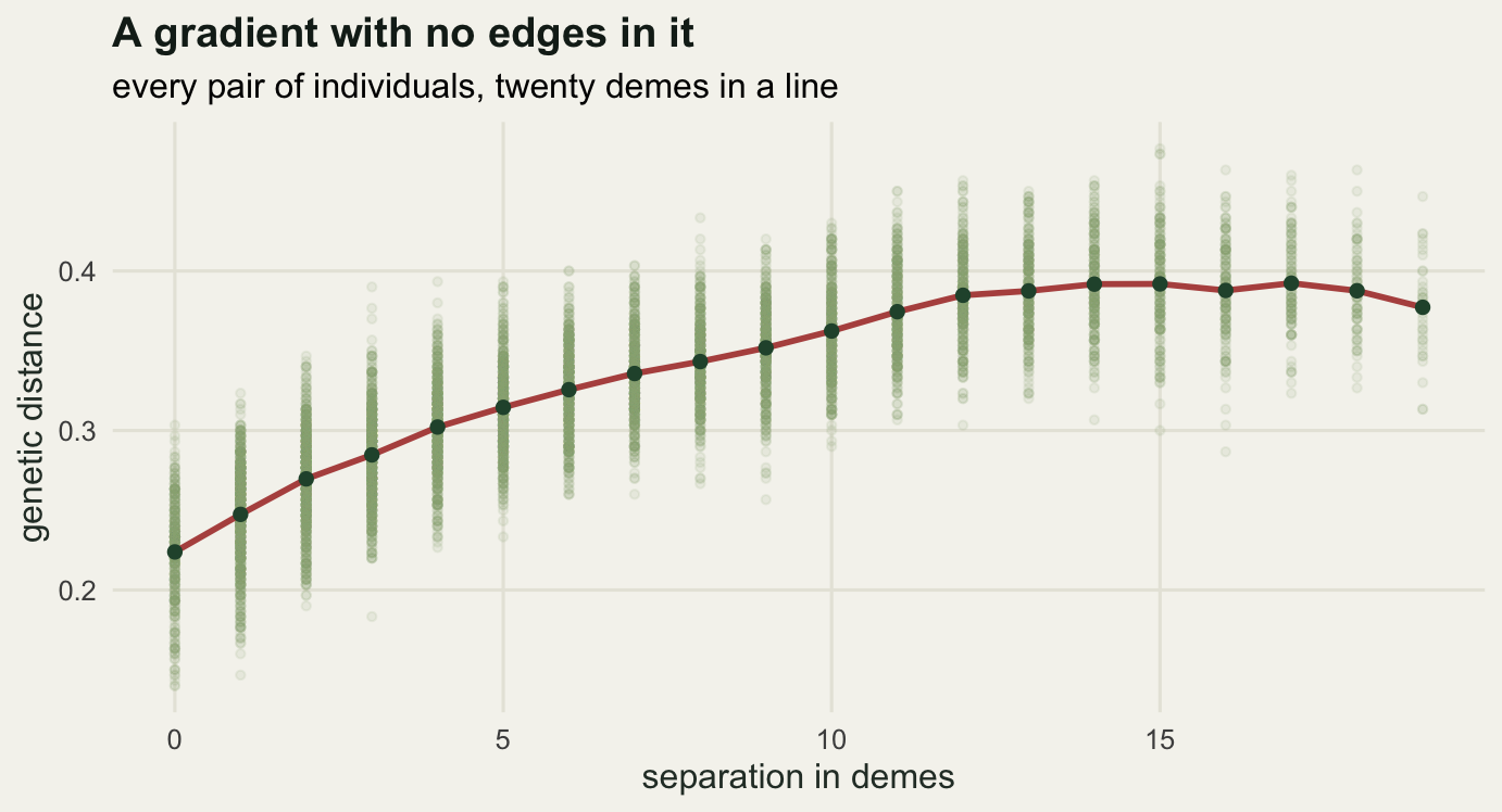
Run the same three criteria on this data set, changing nothing.
crit_two <- criteria(d_two$geno, seed0 = 902)
print(crit_two$tab, row.names = FALSE)
K logLik gain cv_error run_sd delta_k
1 -15864.9 NA 0.89363 0.000 NA
2 -13851.7 2013.2 0.80991 0.717 1589.5
3 -12957.2 894.5 0.77841 28.108 15.2
4 -12438.7 518.5 0.76940 85.544 1.8
5 -12185.6 253.1 0.77938 49.773 0.6
6 -11895.2 290.4 0.77848 59.442 NAOn this run delta K peaks at K = 2 with a value of 1589.5, so the Evanno method reports two populations for a landscape with none. Cross-validation error falls from 0.89363 at K = 1 to a minimum of 0.7694 at K = 4, so cross-validation reports four, though the bottom of that curve is flat enough that the exact K is not firm. The log-likelihood curve gains 2013.2 units at K = 2, 894.5 at K = 3 and 518.5 at K = 4, so its elbow, wherever a reader puts it, is not at one either.
The improvement per added source
The interesting comparison is not which K each criterion picks but how much a new source buys in each case.
n_ent <- length(d_one$geno)
cat("gain per genotype entry from the third source, discrete:",
    round(crit_one$tab$gain[3] / n_ent, 4),
    " cline:", round(crit_two$tab$gain[3] / n_ent, 4), "\n")
gain per genotype entry from the third source, discrete: 0.0108 cline: 0.0497 cat("ratio of those third-source gains, cline over discrete:",
round(crit_two$tab$gain[3] / crit_one$tab$gain[3], 2), "\n")ratio of those third-source gains, cline over discrete: 4.59 cat("cross-validation error spread over K = 3 to 6, cline:",
round(max(crit_two$tab$cv_error[3:6]) - min(crit_two$tab$cv_error[3:6]), 5),
" rise from the best K to K = 6, discrete:",
round(crit_one$tab$cv_error[6] - min(crit_one$tab$cv_error), 5), "\n")cross-validation error spread over K = 3 to 6, cline: 0.00998 rise from the best K to K = 6, discrete: 0.05516 q_cline_2 <- order_src(crit_two$q[[2]])
q_cline_4 <- order_src(crit_two$q[[4]])
cat("percent of individuals whose largest ancestry exceeds 0.9, cline at K = 2:",
round(100 * mean(apply(q_cline_2, 1, max) > 0.9), 2),
" discrete at K = 2:",
round(100 * mean(apply(q_disc, 1, max) > 0.9), 2), "\n")percent of individuals whose largest ancestry exceeds 0.9, cline at K = 2: 50 discrete at K = 2: 40.83 cat("correlation of the first source with cline position, K = 2:",
round(cor(q_cline_2[, 1], d_two$pos), 4),
" K = 4:", round(cor(q_cline_4[, 1], d_two$pos), 4), "\n")correlation of the first source with cline position, K = 2: -0.9661 K = 4: -0.8284 A third source is worth 194.7 log-likelihood units in the data that really has two populations and 894.5 in the cline, a ratio of 4.59. Per genotype entry that is 0.0108 against 0.0497. The extra source in the cline is not a rounding artefact being chased by an overfitting criterion: it earns far more improvement than a spurious third source earns in the discrete data, because in a cline every additional source really does describe part of a real gradient in allele frequencies.
That is why the criteria are not malfunctioning. They are answering the question they were built for, which is whether another source improves the description of the allele frequencies, and in a cline the answer keeps being yes.
Cross-validation is also less decisive here than the discrete case makes it look. Across K = 3 to 6 the error moves by only 0.00998 in the cline, while in the discrete data it rises 0.05516 from its minimum to K = 6. A shallow cross-validation curve is a useful warning sign, and it is the one piece of diagnostic information the three criteria do give away.
long_crit <- function(tab, nm) {
  out <- rbind(data.frame(K = tab$K, value = tab$logLik,
                          crit = "log-likelihood"),
               data.frame(K = tab$K, value = tab$cv_error,
                          crit = "cross-validation"),
               data.frame(K = tab$K, value = tab$delta_k,
                          crit = "Evanno delta K"))
  out$case <- nm
  out[!is.na(out$value), ]
}

crit_df <- rbind(long_crit(crit_one$tab, "discrete: two real sources"),
                 long_crit(crit_two$tab, "continuous: cline of demes"))
crit_df$crit <- factor(crit_df$crit, levels = c("log-likelihood",
                                                "cross-validation",
                                                "Evanno delta K"))
crit_df$case <- factor(crit_df$case, levels = c("discrete: two real sources",
                                                "continuous: cline of demes"))

ggplot(crit_df, aes(K, value)) +
  geom_line(colour = te_pal$sage, linewidth = 0.9) +
  geom_point(colour = te_pal$forest, size = 2.2) +
  facet_grid(crit ~ case, scales = "free_y", switch = "y") +
  scale_x_continuous(breaks = 1:6) +
  labs(title = "Three criteria, two truths",
       subtitle = "identical machinery, five random starts per K",
       x = "number of sources K", y = NULL) +
  theme_te() +
  theme(strip.placement = "outside",
        strip.text.y = element_text(size = 9),
        strip.text.x = element_text(size = 9))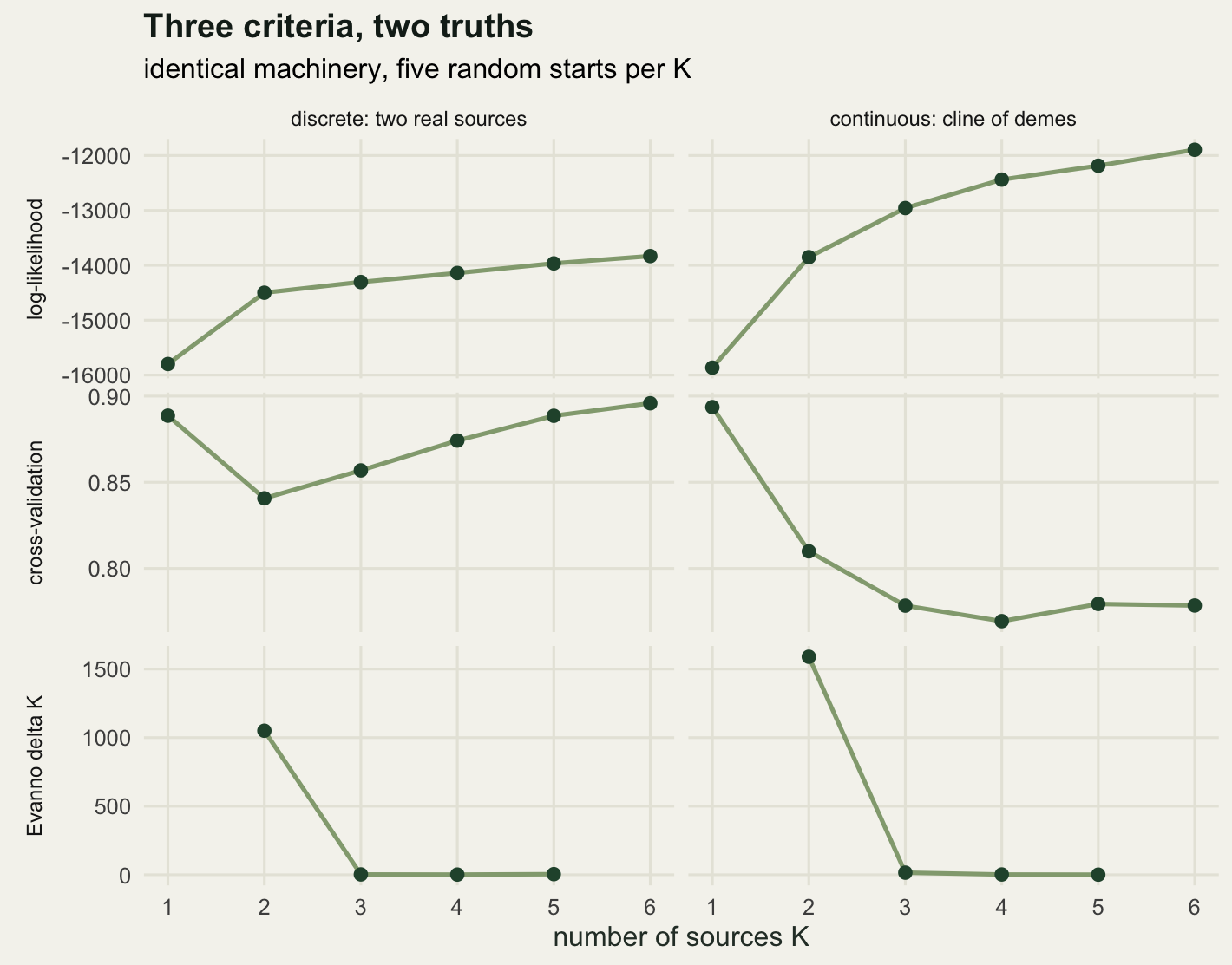
The bar plot readers actually see
None of the numbers above is what appears in a paper. The bar plot is, and the bar plot is where the trouble is.
bar_frame <- function(q_mat, ord, nm) {
  q_mat <- q_mat[ord, , drop = FALSE]
  do.call(rbind, lapply(seq_len(ncol(q_mat)), function(k)
    data.frame(ind = seq_len(nrow(q_mat)), q = q_mat[, k],
               src = paste("source", k), panel = nm)))
}

is_mixed <- d_one$q_true[, 1] < 0.999 & d_one$q_true[, 1] > 0.001
ord_disc <- order(is_mixed, -d_one$q_true[, 1])
ord_cline <- order(d_two$pos)

bars <- rbind(bar_frame(q_disc, ord_disc, "discrete truth, K = 2"),
              bar_frame(q_cline_2, ord_cline, "cline, K = 2 (Evanno choice)"),
              bar_frame(q_cline_4, ord_cline,
                        "cline, K = 4 (cross-validation choice)"))
bars$panel <- factor(bars$panel,
                     levels = c("discrete truth, K = 2",
                                "cline, K = 2 (Evanno choice)",
                                "cline, K = 4 (cross-validation choice)"))

ggplot(bars, aes(ind, q, fill = src)) +
  geom_col(width = 1) +
  facet_wrap(~panel, ncol = 1) +
  scale_fill_manual(values = c(te_pal$forest, te_pal$clay, te_pal$gold,
                               te_pal$sage), name = NULL) +
  scale_y_continuous(expand = c(0, 0)) +
  labs(title = "The same tidy bar plot from two different worlds",
       subtitle = "top panel ordered by group, lower panels by position along the line",
       x = "individual", y = "ancestry") +
  theme_te() +
  theme(panel.grid = element_blank())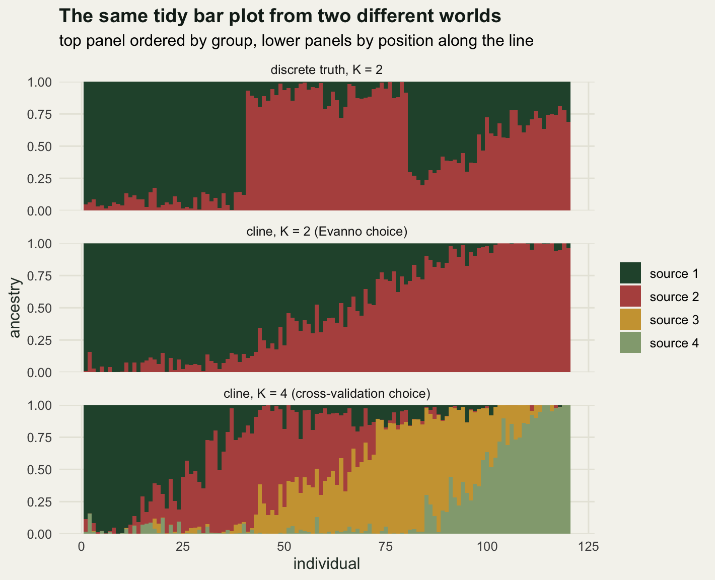
The cline panels are the point. At K = 2, 50 per cent of the individuals have a largest ancestry above 0.9, against 40.83 per cent in the data set that really does contain two populations, so by the usual visual standard the cline looks more cleanly structured than the genuinely structured data. At K = 4 the four sources line up along the line in order, and the leading source correlates with position at -0.9661 for K = 2 and -0.8284 for K = 4. Read as a map of populations, the plot says four groups meeting at three contact zones. Read correctly, it says that allele frequencies change gradually along a line of demes, which the previous figure already showed without any clusters in it.
What the criteria cannot tell you
Three limits, and the first is the one that matters.
Every criterion here compares nested models of the same kind, so each answers “does another source improve the fit of a mixture of discrete allele frequency vectors”. None of them can answer “how many populations exist”, and under continuous variation the second question has no answer to find. A selected K is a model index.
Delta K carries a structural quirk on top of that. It is built from second differences, so it needs K-1, K and K+1, which leaves it undefined at the smallest and the largest K in the range: both tables above print it as NA at K = 1 and K = 6. Delta K therefore cannot select one population, whatever the data look like, and since panmixia is the null in most studies, a statistic that cannot report the null is a strange choice for testing against it. Its size is not interpretable either. The denominator is the run-to-run spread of an optimiser, 1.061 at K = 2 in the discrete data and 0.717 in the cline, and the size of the ratio tracks that spread rather than the strength of the evidence.
Cross-validation on genotype entries assumes the entries are exchangeable, so hiding one and predicting it from the rest is a fair test. Linked loci break that assumption: a hidden entry at a locus tightly linked to an observed one is partly copied rather than predicted, which flatters every K and flatters larger K most. Holding out whole individuals, or whole chromosome blocks, is the more honest design and it is harder to arrange.
What does help
Since K is a model index, the useful questions are not about its value. The first is whether the clusters are spatially coherent in a way a gradient would not produce: a cline gives clusters that are contiguous along the gradient and whose boundaries move when K changes, whereas real barriers give boundaries that stay in the same place across K.
The second is stability. Refit with a random half of the loci, then with a random subset of individuals, and check whether the same individuals stay together. Sampling design leaks directly into the answer, because uneven sampling along a gradient creates apparent clusters at the sampled patches, which is one of the standard ways clines are mistaken for populations.
The third is to fit a model that can represent the alternative. Explicitly spatial methods let allele frequencies vary continuously with geography instead of only through discrete sources, and they can be compared with a discrete-cluster model on the same data: conStruct, SpaceMix, TESS and EEMS all take this route in different ways, and a plain ordination of the genotype matrix will already show a cline as a single dominant axis rather than as clumps. Fitting one of these is the only check in this list that can support the claim that discrete clusters exist rather than assuming them.
Where to go next
The next tutorial in this cluster is the checking post, which takes the diagnostics named above and measures them: how much the bar plot moves when loci and individuals are resampled, what uneven sampling along a gradient does to the apparent number of clusters, and how far the ancestry estimates can be trusted for individuals with little ancestry from any one source.
References
Evanno G, Regnaut S, Goudet J 2005 Molecular Ecology 14(8):2611-2620 (10.1111/j.1365-294X.2005.02553.x)
Kalinowski ST 2011 Heredity 106(4):625-632 (10.1038/hdy.2010.95)
Frantz AC, Cellina S, Krier A, Schley L, Burke T 2009 Journal of Applied Ecology 46(2):493-505 (10.1111/j.1365-2664.2008.01606.x)
Bradburd GS, Coop GM, Ralph PL 2018 Genetics 210(1):33-52 (10.1534/genetics.118.301333)
Janes JK et al 2017 Molecular Ecology 26(14):3594-3602 (10.1111/mec.14187)