library(vegan)
library(ggplot2)

te_paper  <- "#f5f4ee"
te_ink    <- "#16241d"
te_body   <- "#2c3a31"
te_forest <- "#275139"
te_rust   <- "#b5534e"
te_gold   <- "#c9b458"
te_line   <- "#dad9ca"

theme_datasheet <- function() {
  theme_minimal(base_size = 12) +
    theme(plot.background  = element_rect(fill = te_paper, colour = NA),
          panel.background = element_rect(fill = te_paper, colour = NA),
          panel.grid.major = element_line(colour = te_line, linewidth = 0.3),
          panel.grid.minor = element_blank(),
          text             = element_text(colour = te_body),
          plot.title       = element_text(colour = te_ink, face = "bold"),
          plot.subtitle    = element_text(colour = te_body),
          axis.text        = element_text(colour = te_body),
          strip.text       = element_text(colour = te_ink, face = "bold"))
}betadisper with unequal group sizes
R
vegan
PERMANOVA
multivariate
beta diversity
simulation
ecology tutorial
With five plots against fifty, betadisper often finds a dispersion gap that is not there. Testing bias.adjust in R on three distances, and what it leaves.
Five fenced exclosures and fifty grazed plots on the same hill pasture, one season after the fences went up. The fences were expensive and the grazed plots were already part of a monitoring scheme, so the design is five against fifty. The question is whether fencing has changed how different the plots are from one another: the spread of plots around their group’s centre in species space, which Anderson, Ellingsen and McArdle (2006) set out as a measure of beta diversity. In R that is vegan::betadisper() on a dissimilarity matrix, followed by anova() or permutest() on the distances it returns.
This site already insists on that test. Four common PERMANOVA mistakes in ecology makes it compulsory beside every PERMANOVA, and its Mistake 4, on unbalanced groups, tells the reader to treat a significant result with unequal group sizes and unequal dispersions with suspicion, and to lean on the dispersion test to interpret it. Statistics on an ordination and Pairwise PERMANOVA both run betadisper() and read a non-significant result as clearing the PERMANOVA; both do so on groups of equal size, which is the case that turns out below to be safe. None of the three measures the dispersion test itself when the groups are unequal, and that is exactly the situation in which Mistake 4 sends the reader to it.
What happens there is documented. The betadisper() help page says, citing Anderson (2006), that dispersion measured around a centre calculated from the same data is biased downward and that the bias matters most with small, unequal groups, and it offers bias.adjust = TRUE, a square root of n over n minus one correction that it attributes to Stier and colleagues (2013). The default is bias.adjust = FALSE. This post demonstrates that documented behaviour; it does not discover it. It reproduces the size of the shrinkage from a closed form, then measures what the help page does not give: the rejection rates of the default and the adjusted test for three dissimilarities and both kinds of group centre, how far the adjustment falls short, and what the bias does to the check that Mistake 4 recommends.
What the default does, read from the source
Three kinds of community table with twenty five species each cover three dissimilarities in common use. Normal scores with Euclidean distance are the textbook case; presence and absence with a fixed occurrence probability per species goes to binary Jaccard; negative binomial counts go to Bray-Curtis. In every null simulation below both groups are drawn from one and the same distribution, so their true dispersion is equal by construction and every rejection is a false one.
n_spp  <- 25                                           # species in every table
p_occ  <- seq(0.1, 0.7, length.out = n_spp)            # occurrence probabilities
mu_cnt <- exp(seq(log(0.5), log(30), length.out = n_spp))  # mean counts
nb_size <- 1                                           # negative binomial size
n_rep   <- 500   # datasets per cell of the null grid
n_perm  <- 199   # permutations inside every permutest-style test
n_rep_k <- 300   # datasets per point of the blind-spot curve

gen <- list(
  euclidean = function(n) matrix(rnorm(n * n_spp), n, n_spp),
  jaccard   = function(n) matrix(rbinom(n * n_spp, 1, rep(p_occ, each = n)), n, n_spp),
  bray      = function(n) matrix(rnbinom(n * n_spp, size = nb_size,
                                         mu = rep(mu_cnt, each = n)), n, n_spp))
dist_fun <- list(euclidean = function(y) dist(y),
                 jaccard   = function(y) vegdist(y, "jaccard", binary = TRUE),
                 bray      = function(y) vegdist(y, "bray"))
dist_lab <- c(euclidean = "Euclidean, normal scores",
              jaccard   = "Jaccard, presence-absence",
              bray      = "Bray-Curtis, counts")

make_groups <- function(n_small, n_large)
  factor(rep(c("small", "large"), c(n_small, n_large)), levels = c("small", "large"))

# betadisper, counting (not printing) its warning about negative squared distances
n_neg_warn <- 0; n_fits <- 0
disper <- function(d, grp, ...) withCallingHandlers({
  n_fits <<- n_fits + 1
  betadisper(d, grp, ...)
},
  warning = function(w) {
    if (grepl("negative and changed to zero", conditionMessage(w))) {
      n_neg_warn <<- n_neg_warn + 1
      invokeRestart("muffleWarning")
    }
  })

# distances to the group centroid, from the PCoA axes betadisper already built
centroid_dist <- function(bd) {
  pos <- bd$eig > 0
  cen <- rowsum(bd$vectors, bd$group) / as.vector(table(bd$group))
  dev <- bd$vectors - cen[as.integer(bd$group), , drop = FALSE]
  sqrt(pmax(rowSums(dev[, pos, drop = FALSE]^2) -
            rowSums(dev[, !pos, drop = FALSE]^2), 0))
}
adj_factor <- function(grp) {
  n_g <- as.vector(table(grp))
  sqrt(n_g[grp] / (n_g[grp] - 1))
}set.seed(4101)
y_chk <- rbind(gen$bray(5), gen$bray(50))
g_chk <- make_groups(5, 50)
d_chk <- dist_fun$bray(y_chk)
bd_def <- disper(d_chk, g_chk)
bd_adj <- disper(d_chk, g_chk, bias.adjust = TRUE)
bd_cen <- disper(d_chk, g_chk, type = "centroid")
bd_cen_adj <- disper(d_chk, g_chk, type = "centroid", bias.adjust = TRUE)
# the defaults, as the fitted object records them
stopifnot(identical(formals(betadisper)$bias.adjust, FALSE),
attr(bd_def, "type") == "median",
identical(attr(bd_def, "bias.adjust"), FALSE),
formals(getS3method("permutest", "betadisper"))$permutations == 999)
# bias.adjust multiplies every distance by sqrt(n / (n - 1)) of its own group, for both types
gap_adj_med <- max(abs(bd_adj$distances - bd_def$distances * adj_factor(g_chk)))
gap_adj_cen <- max(abs(bd_cen_adj$distances - bd_cen$distances * adj_factor(g_chk)))
# the hand centroid distances reproduce type = "centroid"
gap_cen <- max(abs(centroid_dist(bd_def) - bd_cen$distances))
# anova() is a one-way linear model on the distances
p_hand <- summary(lm(bd_def$distances ~ g_chk))$coefficients[2, 4]
gap_anova <- abs(p_hand - anova(bd_def)$`Pr(>F)`[1])
stopifnot(gap_adj_med < 1e-12, gap_adj_cen < 1e-12, gap_cen < 1e-10, gap_anova < 1e-10)
ver_vegan <- packageDescription("vegan")$VersionThe defaults are read from the fitted object rather than from memory. On vegan 2.7-5, the version installed here, bias.adjust is FALSE, the type is the spatial median and permutest() uses 999 permutations; the development source on GitHub (vegan 2.8-0, read on 26 September 2026) has the same three defaults and the same adjustment line. The adjustment is applied as the source applies it: every distance is multiplied by the square root of n over n minus one for its own group, for the median and the centroid alike, and the chunk checks that the adjusted objects equal the default distances times that factor within \(10^{-12}\). anova() on a betadisper object is a one-way linear model on the distances, and its p value matches lm() to within floating-point rounding. The simulations below take centroid distances from the principal coordinates that the median fit has already built, which reproduces type = "centroid" to within floating-point rounding and saves a second fit per dataset.
Five exclosures against fifty grazed plots
Ten simulated pastures, each with five fenced and fifty grazed plots drawn from the same Bray-Curtis count model, each tested twice: once with the default and once with bias.adjust = TRUE.
n_small <- 5; n_large <- 50
n_draw <- 10
set.seed(4102)
worked <- lapply(seq_len(n_draw), function(i) {
  y <- rbind(gen$bray(n_small), gen$bray(n_large))
  bd <- disper(dist_fun$bray(y), make_groups(n_small, n_large))
  list(bd = bd, p_def = anova(bd)$`Pr(>F)`[1],
       p_adj = anova(disper(dist_fun$bray(y), make_groups(n_small, n_large),
                            bias.adjust = TRUE))$`Pr(>F)`[1])
})
p_def_w <- vapply(worked, `[[`, 0, "p_def")
p_adj_w <- vapply(worked, `[[`, 0, "p_adj")
n_rej_def_w <- sum(p_def_w < 0.05); n_rej_adj_w <- sum(p_adj_w < 0.05)
rej_low_w <- sum(vapply(worked, function(w) w$p_def < 0.05 &&
  w$bd$group.distances["small"] < w$bd$group.distances["large"], TRUE))
bd1 <- worked[[1]]$bd
gd1 <- bd1$group.distances
round(rbind(default = p_def_w, adjusted = p_adj_w), 3)
[,1] [,2] [,3] [,4] [,5] [,6] [,7] [,8] [,9] [,10]
default 0.057 0.703 0.035 0.288 0.415 0.000 0.045 0.188 0.417 0.642
adjusted 0.485 0.352 0.369 0.924 0.768 0.006 0.453 0.788 0.641 0.392In the first pasture the five fenced plots sit on average 0.317 from their median and the fifty grazed plots 0.371, and the default test gives p = 0.057. With the adjustment the same data give p = 0.485. Across the ten pastures the default rejects at 0.05 in 3 and the adjusted test in 1, and in all of the default’s rejections the fenced plots are the tighter group. Ten draws are an anecdote; the rates come further down.
ver_lev <- c("default", "bias.adjust = TRUE")
w1_long <- data.frame(group = factor(rep(bd1$group, 2), labels = c("5 fenced", "50 grazed")),
                      z = c(bd1$distances, bd1$distances * adj_factor(bd1$group)),
                      version = factor(rep(ver_lev, each = length(bd1$group)), levels = ver_lev))
w1_mean <- aggregate(z ~ group + version, data = w1_long, FUN = mean)
set.seed(4103)
ggplot(w1_long, aes(group, z)) +
  geom_jitter(width = 0.12, height = 0, colour = te_body, alpha = 0.6, size = 1.6) +
  geom_crossbar(data = w1_mean, aes(ymin = z, ymax = z), width = 0.5,
                colour = te_rust, linewidth = 0.5) +
  facet_wrap(~ version) +
  labs(x = NULL, y = "distance to group median",
       title = "One pasture, same count model in both groups",
       subtitle = "bars: group mean distance") +
  theme_datasheet()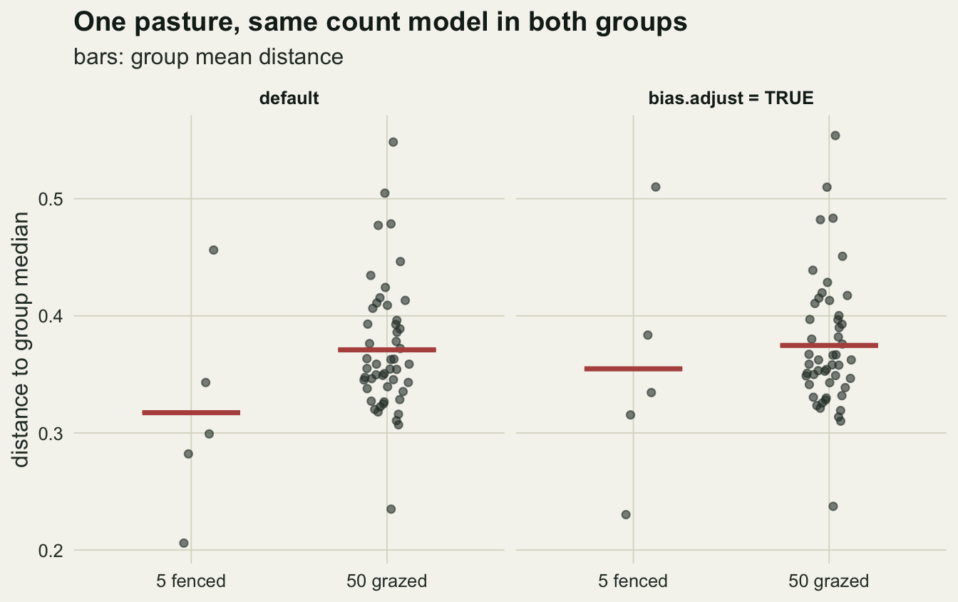
Where the shrinkage comes from
Take n plots drawn independently from a distribution with centre mu and covariance matrix Sigma, and measure each plot’s squared distance to the centroid of the same n plots. The deviation x_i - xbar is (1 - 1/n) (x_i - mu) minus the sum of the other n - 1 deviations (x_j - mu) divided by n. The two parts are independent, so their variances add: (1 - 1/n)^2 + (n - 1) / n^2, which is (n - 1) / n. The expected squared distance to the centroid is therefore (n - 1) / n times tr(Sigma), the expected squared distance to the true centre. The centroid is pulled towards the plots it is computed from; with five plots the pull removes a fifth of the expected squared distance, with fifty it removes a fiftieth.
shrink <- function(n) sqrt((n - 1) / n)
ratio_cf <- function(n1, n2) shrink(n1) / shrink(n2)
pairs_n <- list(c(5, 50), c(8, 32), c(12, 12))
pair_lab <- vapply(pairs_n, function(nn) sprintf("%d vs %d", nn[1], nn[2]), "")
cf_550 <- ratio_cf(5, 50); cf_832 <- ratio_cf(8, 32)
blind_k <- 1 / cf_550
The distance itself is the square root, so when distances are concentrated, as they are with twenty five species, the mean distance shrinks by close to sqrt((n - 1) / n). Under equal true dispersion the ratio of the small group’s mean distance to the large group’s is then sqrt((n1 - 1) / n1) / sqrt((n2 - 1) / n2): 0.904 for five against fifty and 0.950 for eight against thirty two. bias.adjust = TRUE multiplies by the inverse of the centroid factor. The spatial median, the default centre, has no such formula, and vegan applies the same factor to it; how well that borrowed correction works for the median is measured below, not derived.
The rejection rate by design, distance and type
Each cell of the grid is 500 simulated datasets, a number fixed before any rate was looked at, for three pairs of group sizes: five against fifty, eight against thirty two, and a balanced twelve against twelve. Every dataset gets four tests, median and centroid, each with and without the adjustment, and every test is read two ways: the F test that anova() prints, and a permutation test built the way permutest() builds it, by permuting the residuals of the one-way model, with 199 permutations. The hand version reproduces permutest() exactly on a shared permutation matrix; the chunk stops if the two p values differ by more than \(10^{-12}\).
eps_p  <- sqrt(.Machine$double.eps)

# one F test and one residual-permutation test (permutest's scheme) on distances z
two_tests <- function(z, is_small, perm) {
  n1 <- sum(is_small); n_tot <- length(z); n2 <- n_tot - n1
  m1 <- mean(z[is_small]); m2 <- mean(z[!is_small])
  res <- z - ifelse(is_small, m1, m2)
  rss <- sum(res^2)
  mss0 <- n1 * (m1 - mean(z))^2 + n2 * (m2 - mean(z))^2
  f0 <- mss0 / (rss / (n_tot - 2))
  s1 <- rowSums(matrix(res[perm], nrow = nrow(perm))[, is_small, drop = FALSE])
  mss_p <- s1^2 / n1 + s1^2 / n2
  f_p <- mss_p / ((rss - mss_p) / (n_tot - 2))
  c(p_f = pf(f0, 1, n_tot - 2, lower.tail = FALSE),
    p_perm = (sum(f_p >= f0 - eps_p) + 1) / (n_perm + 1),
    diff = m1 - m2, se = sqrt(rss / (n_tot - 2) * (1 / n1 + 1 / n2)),
    m1 = m1, m2 = m2, msq1 = mean(z[is_small]^2), msq2 = mean(z[!is_small]^2))
}
# the hand permutation test reproduces permutest() on the same permutation matrix
set.seed(4104)
perm_chk <- t(replicate(n_perm, sample.int(length(g_chk))))
gap_perm <- abs(permutest(bd_def, permutations = perm_chk)$tab$`Pr(>F)`[1] -
                two_tests(bd_def$distances, g_chk == "small", perm_chk)["p_perm"])
stopifnot(gap_perm < 1e-12)

variants <- c("median, default", "median, adjusted", "centroid, default", "centroid, adjusted")
one_dataset <- function(dname, n1, n2) {
  grp <- make_groups(n1, n2)
  y <- rbind(gen[[dname]](n1), gen[[dname]](n2))
  stopifnot(dname == "euclidean" || all(rowSums(y) > 0))
  bd <- disper(dist_fun[[dname]](y), grp)
  z_cen <- centroid_dist(bd); a_f <- adj_factor(grp)
  perm <- t(replicate(n_perm, sample.int(n1 + n2)))
  sm <- grp == "small"
  rbind(two_tests(bd$distances, sm, perm), two_tests(bd$distances * a_f, sm, perm),
        two_tests(z_cen, sm, perm), two_tests(z_cen * a_f, sm, perm))
}
set.seed(4105)
grid_raw <- list()
for (dn in names(gen)) for (k in seq_along(pairs_n)) {
  nn <- pairs_n[[k]]
  reps <- lapply(seq_len(n_rep), function(i) one_dataset(dn, nn[1], nn[2]))
  arr <- simplify2array(reps)            # variant x statistic x replicate
  grid_raw[[paste(dn, k)]] <- list(dist = dn, pair = pair_lab[k], n1 = nn[1], n2 = nn[2], arr = arr)
}
rates <- do.call(rbind, lapply(grid_raw, function(cell) {
a <- cell$arr
do.call(rbind, lapply(seq_along(variants), function(v) {
dd <- a[v, "diff", ]; se <- a[v, "se", ]
data.frame(dist = cell$dist, pair = cell$pair, n1 = cell$n1, n2 = cell$n2,
variant = variants[v],
type = factor(sub(",.*", "", variants[v]), levels = c("median", "centroid")),
adjust = sub(".*, ", "", variants[v]),
rej_f = mean(a[v, "p_f", ] < 0.05), rej_perm = mean(a[v, "p_perm", ] < 0.05),
ratio = mean(a[v, "m1", ]) / mean(a[v, "m2", ]),
msq_ratio = mean(a[v, "msq1", ]) / mean(a[v, "msq2", ]),
shift_sd = mean(dd) / sd(dd), sd_ratio = sd(dd) / sqrt(mean(se^2)))
}))
}))
rates$pair <- factor(rates$pair, levels = pair_lab)
rates$dist_f <- factor(dist_lab[rates$dist], levels = dist_lab)
rates$mcse_f <- sqrt(rates$rej_f * (1 - rates$rej_f) / n_rep)
mcse_05 <- sqrt(0.05 * 0.95 / n_rep)
rate <- function(dn, pr, vr, col = "rej_f")
rates[rates$dist == dn & rates$pair == pr & rates$variant == vr, col]
# balanced cells: the adjustment multiplies every distance by the same factor
bal <- rates[rates$pair == "12 vs 12", ]
stopifnot(all(abs(bal$rej_f[bal$adjust == "default"] - bal$rej_f[bal$adjust == "adjusted"]) < 1e-12))
rng <- function(pr, adj, ty = c("median", "centroid"), col = "rej_f")
range(rates[rates$pair %in% pr & rates$adjust == adj & rates$type %in% ty, col])
range_def550 <- rng("5 vs 50", "default"); range_adj550 <- rng("5 vs 50", "adjusted")
range_perm_def550 <- rng("5 vs 50", "default", col = "rej_perm")
thesis_gap <- rng("5 vs 50", "default", "median")[1] - 0.05
range_def832 <- rng("8 vs 32", "default"); range_adj832 <- rng("8 vs 32", "adjusted")
adj550_med <- rng("5 vs 50", "adjusted", "median"); adj550_cen <- rng("5 vs 50", "adjusted", "centroid")
bal_range <- rng("12 vs 12", "default"); bal_med <- rng("12 vs 12", "default", "median")
bal_cen <- rng("12 vs 12", "default", "centroid")
bal_dev_se <- max(abs(bal$rej_f - 0.05)) / mcse_05
perm_gap <- max(abs(rates$rej_perm - rates$rej_f))
adj_unb <- rates[rates$pair != "12 vs 12" & rates$adjust == "adjusted", ]
cen_minus_med <- adj_unb$rej_f[adj_unb$type == "centroid"] - adj_unb$rej_f[adj_unb$type == "median"]
stopifnot(all(cen_minus_med > 0))
tab_rates <- rates[rates$pair != "12 vs 12" | rates$adjust == "default",
c("dist_f", "pair", "variant", "rej_f", "rej_perm")]
knitr::kable(tab_rates, digits = 3, row.names = FALSE,
col.names = c("dissimilarity", "groups", "centre and setting", "F test", "permutation"))| dissimilarity | groups | centre and setting | F test | permutation |
|---|---|---|---|---|
| Euclidean, normal scores | 5 vs 50 | median, default | 0.308 | 0.280 |
| Euclidean, normal scores | 5 vs 50 | median, adjusted | 0.066 | 0.060 |
| Euclidean, normal scores | 5 vs 50 | centroid, default | 0.320 | 0.298 |
| Euclidean, normal scores | 5 vs 50 | centroid, adjusted | 0.080 | 0.074 |
| Euclidean, normal scores | 8 vs 32 | median, default | 0.130 | 0.122 |
| Euclidean, normal scores | 8 vs 32 | median, adjusted | 0.058 | 0.054 |
| Euclidean, normal scores | 8 vs 32 | centroid, default | 0.164 | 0.144 |
| Euclidean, normal scores | 8 vs 32 | centroid, adjusted | 0.068 | 0.060 |
| Euclidean, normal scores | 12 vs 12 | median, default | 0.032 | 0.034 |
| Euclidean, normal scores | 12 vs 12 | centroid, default | 0.052 | 0.042 |
| Jaccard, presence-absence | 5 vs 50 | median, default | 0.222 | 0.212 |
| Jaccard, presence-absence | 5 vs 50 | median, adjusted | 0.060 | 0.052 |
| Jaccard, presence-absence | 5 vs 50 | centroid, default | 0.242 | 0.242 |
| Jaccard, presence-absence | 5 vs 50 | centroid, adjusted | 0.084 | 0.080 |
| Jaccard, presence-absence | 8 vs 32 | median, default | 0.116 | 0.100 |
| Jaccard, presence-absence | 8 vs 32 | median, adjusted | 0.052 | 0.046 |
| Jaccard, presence-absence | 8 vs 32 | centroid, default | 0.140 | 0.122 |
| Jaccard, presence-absence | 8 vs 32 | centroid, adjusted | 0.070 | 0.060 |
| Jaccard, presence-absence | 12 vs 12 | median, default | 0.044 | 0.030 |
| Jaccard, presence-absence | 12 vs 12 | centroid, default | 0.060 | 0.058 |
| Bray-Curtis, counts | 5 vs 50 | median, default | 0.232 | 0.230 |
| Bray-Curtis, counts | 5 vs 50 | median, adjusted | 0.078 | 0.078 |
| Bray-Curtis, counts | 5 vs 50 | centroid, default | 0.258 | 0.246 |
| Bray-Curtis, counts | 5 vs 50 | centroid, adjusted | 0.102 | 0.094 |
| Bray-Curtis, counts | 8 vs 32 | median, default | 0.134 | 0.126 |
| Bray-Curtis, counts | 8 vs 32 | median, adjusted | 0.064 | 0.054 |
| Bray-Curtis, counts | 8 vs 32 | centroid, default | 0.156 | 0.152 |
| Bray-Curtis, counts | 8 vs 32 | centroid, adjusted | 0.080 | 0.072 |
| Bray-Curtis, counts | 12 vs 12 | median, default | 0.032 | 0.028 |
| Bray-Curtis, counts | 12 vs 12 | centroid, default | 0.052 | 0.050 |
At five against fifty the default rejects a true null in 0.222 to 0.320 of datasets with the F test, depending on the dissimilarity and the type, and in 0.212 to 0.298 with the permutation test. The Monte Carlo standard error of a rate at the nominal level is 0.0097, and even the lowest of the default median cells sits 0.172 above 0.05. At eight against thirty two the default rejects in 0.116 to 0.164. Switching to permutest() does not help: across all cells its rate is within 0.028 of the F test’s. It permutes the residuals of the same model, so the observed F still carries the shift and the permuted ones do not.
With the adjustment, five against fifty drops to 0.060 to 0.102 with the F test: 0.060 to 0.078 for the median and 0.080 to 0.102 for the centroid. At eight against thirty two the adjusted range is 0.052 to 0.080. So the adjustment removes most of the excess, and it leaves more of it with the centroid than with the median in every one of the six unbalanced pairings of design and dissimilarity. In the balanced design the adjustment multiplies every distance by the same constant and changes nothing, which the chunk checks; the balanced rates run from 0.032 to 0.060 (median 0.032 to 0.044, centroid 0.052 to 0.060), and the largest departure from 0.05 is 1.8 Monte Carlo standard errors.
gl <- rbind(data.frame(rates[, c("dist", "pair", "type", "adjust")], rate = rates$rej_f,
                       test = "anova(), F test"),
            data.frame(rates[, c("dist", "pair", "type", "adjust")], rate = rates$rej_perm,
                       test = "permutest(), 199 permutations"))
gl$mcse <- sqrt(gl$rate * (1 - gl$rate) / n_rep)
gl$dist <- factor(dist_lab[gl$dist], levels = dist_lab)
gl$adjust <- factor(gl$adjust, levels = c("default", "adjusted"),
                    labels = c("default", "bias.adjust = TRUE"))
gl$type <- factor(gl$type, levels = c("median", "centroid"))
ggplot(gl, aes(pair, rate, colour = adjust, shape = type,
               group = interaction(adjust, type))) +
  geom_hline(yintercept = 0.05, linetype = "dashed", colour = te_body, linewidth = 0.5) +
  geom_errorbar(aes(ymin = rate - 2 * mcse, ymax = rate + 2 * mcse),
                width = 0, linewidth = 0.4, position = position_dodge(width = 0.6)) +
  geom_point(size = 2.3, position = position_dodge(width = 0.6)) +
  facet_grid(test ~ dist) +
  scale_colour_manual(values = c(te_rust, te_forest), name = NULL) +
  scale_shape_manual(values = c(16, 17), name = NULL) +
  scale_y_continuous(limits = c(0, NA)) +
  labs(x = "group sizes, small vs large", y = "rejection rate, equal true dispersion",
       title = "Equal true dispersion: the default rejects too often",
       subtitle = "dashed line: nominal 0.05; bars: two Monte Carlo standard errors") +
  theme_datasheet() + theme(legend.position = "bottom")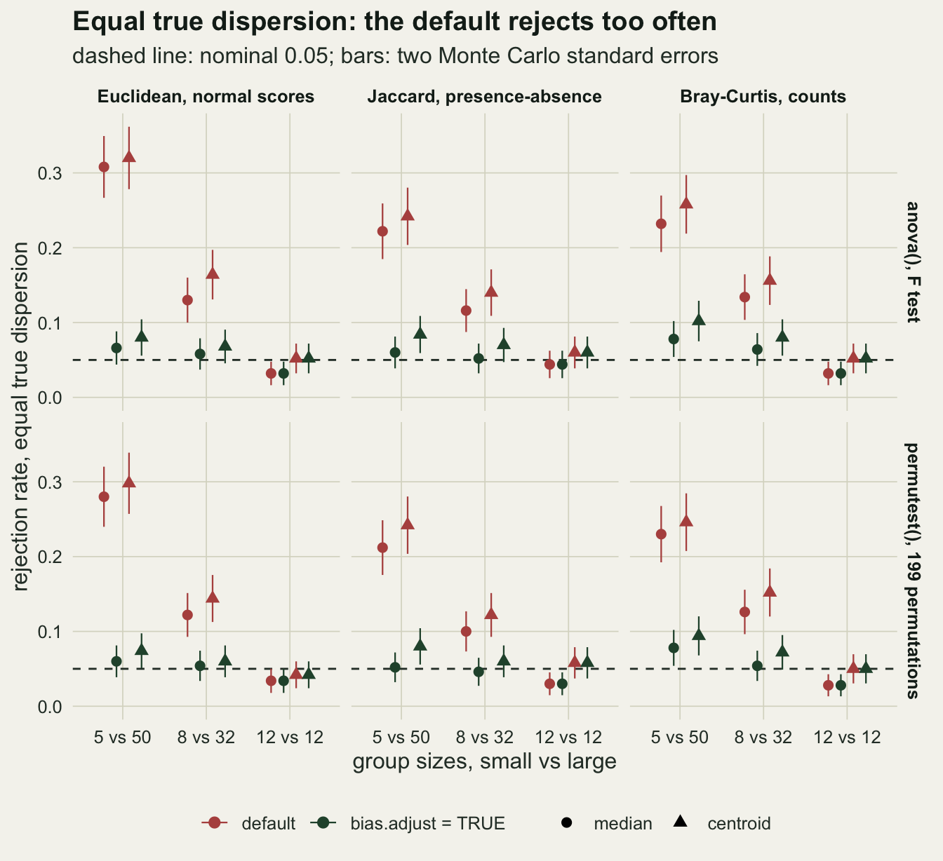
What the adjustment fixes and what it leaves
Two separate things can make an F test on distances reject too often. The small group’s mean distance can be shifted relative to the large group’s, which is what the closed form describes. Or the difference between the two group means can vary more from dataset to dataset than the F test’s standard error allows, and that second excess can come from the correction itself. The simulations record both: the average difference in units of its own standard deviation across datasets, and the ratio of that standard deviation to the root mean square of the F test’s standard error.
eu <- rates[rates$dist == "euclidean" & rates$variant == "centroid, default", ]
msq_cf <- ((eu$n1 - 1) / eu$n1) / ((eu$n2 - 1) / eu$n2)
gap_msq <- max(abs(eu$msq_ratio - msq_cf))
unb <- rates[rates$pair != "12 vs 12", ]
unb_d <- unb[unb$adjust == "default", ]
gap_ratio <- max(abs(unb_d$ratio - ratio_cf(unb_d$n1, unb_d$n2)))
shift_def <- range(rates$shift_sd[rates$pair == "5 vs 50" & rates$adjust == "default"])
shift_adj <- range(rates$shift_sd[rates$pair == "5 vs 50" & rates$adjust == "adjusted"])
sdr_adj <- range(rates$sd_ratio[rates$pair == "5 vs 50" & rates$adjust == "adjusted"])
unb_a <- unb[unb$adjust == "adjusted", ]
unb_a$approx <- 2 * pnorm(-qnorm(0.975) / unb_a$sd_ratio)
gap_approx <- max(abs(unb_a$approx - unb_a$rej_f))
worst <- unb_a[which.max(unb_a$rej_f), ]
worst_lab <- c(euclidean = "Euclidean", jaccard = "Jaccard", bray = "Bray-Curtis")[[worst$dist]]

# what the adjustment does to the spread: the design factor, if the default distances vary
# equally within the two groups (variance of a group mean ~ 1 / n_g, pooled RSS weighted by df)
mult_cf <- function(n1, n2)
  sqrt((1 / (n1 - 1) + 1 / (n2 - 1)) / (1 / n1 + 1 / n2) * (n1 + n2 - 2) / (n1 + n2))
var_cf <- function(n1, n2) (1 / (n1 - 1) + 1 / (n2 - 1)) / (1 / n1 + 1 / n2)
se2_cf <- function(n1, n2) (n1 + n2) / (n1 + n2 - 2)
stopifnot(identical(unb_a$dist, unb_d$dist), identical(unb_a$pair, unb_d$pair),
          identical(unb_a$type, unb_d$type),
          isTRUE(all.equal(mult_cf(5, 50)^2, var_cf(5, 50) / se2_cf(5, 50))))
gap_mult <- max(abs(unb_a$sd_ratio / unb_d$sd_ratio - mult_cf(unb_a$n1, unb_a$n2)))
# the two ingredients, from the same datasets (variants 1, 2 = median; 3, 4 = centroid)
ingr <- do.call(rbind, lapply(grid_raw[vapply(grid_raw, `[[`, "", "pair") != "12 vs 12"],
  function(cell) {
    a <- cell$arr
    data.frame(n1 = cell$n1, n2 = cell$n2,
               var_up = c(var(a[2, "diff", ]) / var(a[1, "diff", ]),
                          var(a[4, "diff", ]) / var(a[3, "diff", ])),
               se2_up = c(mean(a[2, "se", ]^2) / mean(a[1, "se", ]^2),
                          mean(a[4, "se", ]^2) / mean(a[3, "se", ]^2)))
  }))
i550 <- ingr$n1 == 5
var_up550 <- range(ingr$var_up[i550]); se2_up550 <- range(ingr$se2_up[i550])
d550 <- unb_d[unb_d$pair == "5 vs 50", ]
sdr_def_med <- range(d550$sd_ratio[d550$type == "median"])
sdr_def_cen <- range(d550$sd_ratio[d550$type == "centroid"])
a550 <- unb_a[unb_a$pair == "5 vs 50", ]
sdr_adj_med <- range(a550$sd_ratio[a550$type == "median"])
sdr_adj_cen <- range(a550$sd_ratio[a550$type == "centroid"])
# with the median, most of the adjusted excess over 1 is added by the correction
share_med <- ((a550$sd_ratio - d550$sd_ratio) / (a550$sd_ratio - 1))[a550$type == "median"]
stopifnot(all(a550$sd_ratio > 1), all(share_med > 0.5))
# same factor for both types, so the centroid leaves more wherever its default ratio is higher
stopifnot(all(unb_d$sd_ratio[unb_d$type == "centroid"] > unb_d$sd_ratio[unb_d$type == "median"]))
The closed form first. For Euclidean distances to the centroid the squared-distance result is exact, and the simulated ratio of mean squared distances matches (n1 - 1) / n1 over (n2 - 1) / n2 to within 0.0048 in all three designs. For mean distances, in every unbalanced cell, for both types and all three dissimilarities, the average small-group mean distance over the average large-group one is within 0.0075 of the square root version. The Jaccard and Bray-Curtis tables shrink the way the textbook case does, and the median shrinks by about as much as the centroid.
shr <- rates[rates$adjust == "default", ]
shr_cf <- data.frame(pair = factor(pair_lab, levels = pair_lab),
                     cf = vapply(pairs_n, function(nn) ratio_cf(nn[1], nn[2]), 0))
ggplot(shr, aes(pair, ratio)) +
  geom_errorbar(data = shr_cf, aes(x = pair, ymin = cf, ymax = cf), inherit.aes = FALSE,
                width = 0.75, colour = te_body, linewidth = 0.6, linetype = "dashed") +
  geom_point(aes(colour = dist_f, shape = type, group = interaction(dist_f, type)),
             size = 2.6, position = position_dodge(width = 0.6)) +
  scale_colour_manual(values = c(te_forest, te_gold, te_rust), name = NULL) +
  scale_shape_manual(values = c(16, 17), name = NULL) +
  labs(x = "group sizes, small vs large", y = "mean distance ratio, small / large",
       title = "Default: the shrinkage follows the closed form",
       subtitle = "dashed bars: sqrt((n1 - 1) / n1) / sqrt((n2 - 1) / n2)") +
  theme_datasheet() + theme(legend.position = "bottom", legend.box = "vertical")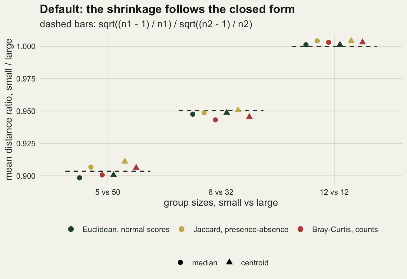
At five against fifty the default’s average difference between the small and the large group lies between 1.11 and 1.47 of its own standard deviations below zero. After the adjustment it lies between -0.075 and 0.107: almost all of the shift is gone. What survives is spread, and it is not simply left over from the default. At five against fifty the default’s own ratio of the spread of the difference to the F test’s standard error is 0.97 to 1.03 with the median and 1.03 to 1.10 with the centroid; adjusted it is 1.05 to 1.12 and 1.12 to 1.19. With the median most of the excess over 1 is added by the correction; with the centroid part of it was there before. Multiplying the five distances by the square root of 5/4 multiplies the variance of their mean by 5/4, while the pooled variance behind the F test’s standard error, set mostly by the fifty, grows only by about n / (n - 2). If the default distances vary about equally within the two groups, the ratio therefore grows by
sqrt((1 / (n1 - 1) + 1 / (n2 - 1)) / (1 / n1 + 1 / n2) * (n - 2) / n),
which is 1.088 for five against fifty and 1.032 for eight against thirty two. On the same datasets the variance of the difference grew by 1.231 to 1.232 at five against fifty, against 1.229 from the first part of the formula, and the mean squared standard error by 1.034 to 1.049, against 1.038. The factor reproduces the adjusted ratio over the default one within 0.0050 in all twelve unbalanced cells. It is the same for both types, so the centroid leaves more than the median because its default ratio was already higher, which holds in all six unbalanced pairings.
A test whose standard error is too small by a factor r rejects at about 2 * pnorm(-1.96 / r) when the statistic is close to normal. That one line reproduces the adjusted rates of all twelve unbalanced cells to within 0.0063. The worst cell, Bray-Curtis with the centroid, has a ratio of 1.19 and rejects in 0.102 of datasets.
sd_grid <- data.frame(sd_ratio = seq(0.95, 1.3, by = 0.005))
sd_grid$approx <- 2 * pnorm(-qnorm(0.975) / sd_grid$sd_ratio)
unb_a$sd_ratio_def <- unb_d$sd_ratio
ggplot(unb_a, aes(sd_ratio, rej_f)) +
  geom_segment(aes(x = sd_ratio_def, xend = sd_ratio, y = rej_f, yend = rej_f, colour = dist_f),
               linewidth = 0.35, show.legend = FALSE) +
  geom_point(aes(x = sd_ratio_def, colour = dist_f), size = 2.2, show.legend = FALSE,
             shape = ifelse(unb_a$type == "median", 1, 2)) +      # hollow: default ratio
  geom_line(data = sd_grid, aes(sd_ratio, approx), colour = te_body, linewidth = 0.6,
            linetype = "dotted", inherit.aes = FALSE) +
  geom_hline(yintercept = 0.05, linetype = "dashed", colour = te_body, linewidth = 0.5) +
  geom_errorbar(aes(ymin = rej_f - 2 * mcse_f, ymax = rej_f + 2 * mcse_f,
                    colour = dist_f), width = 0, linewidth = 0.4, show.legend = FALSE) +
  geom_point(aes(colour = dist_f, shape = type), size = 2.6) +
  scale_colour_manual(values = c(te_forest, te_gold, te_rust), name = NULL) +
  scale_shape_manual(values = c(16, 17), name = NULL) +
  labs(x = "SD of the group difference / F test standard error",
       y = "rejection rate, bias.adjust = TRUE",
       title = "Adjusted: the correction stretches the small group",
       subtitle = "dotted: 2 * pnorm(-1.96 / ratio); dashed: 0.05; bars: two Monte Carlo SE") +
  theme_datasheet() + theme(legend.position = "bottom", legend.box = "vertical")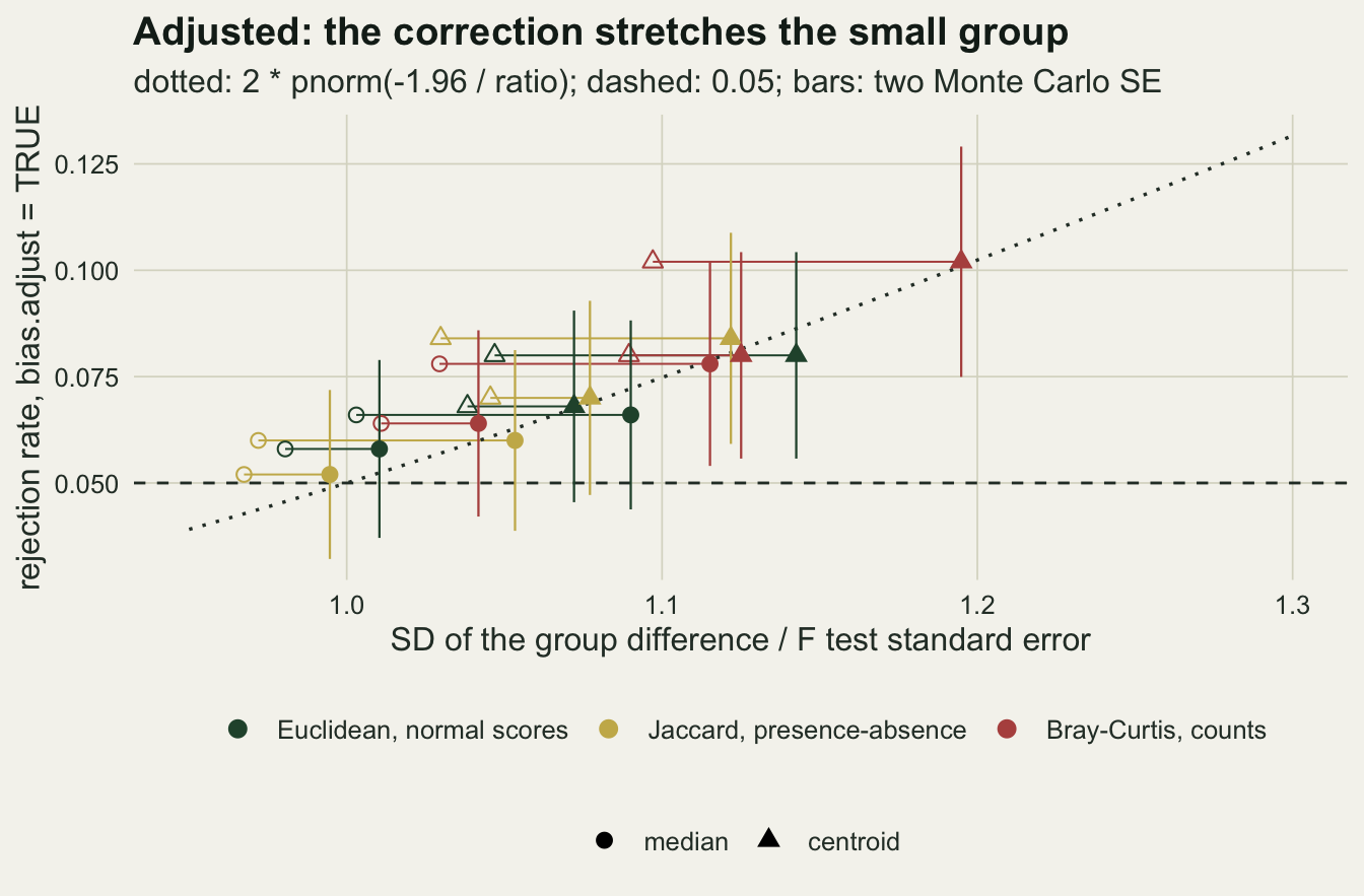
The blind spot sits where Mistake 4 looks
Mistake 4 of the PERMANOVA post, following Anderson and Walsh (2013), warns that an unbalanced PERMANOVA is too liberal when the smaller group is the more dispersed one, and the reader who takes its advice runs betadisper() to find out whether that is the case. The shrinkage works against that reader. The default sees the small group’s dispersion multiplied by about 0.904, so a small group that is truly more dispersed by the inverse of that factor, 1.107, looks exactly as dispersed as the large one. The closed form puts the default’s blind spot there, not at equal dispersion. To look at it, the five plots are drawn with their scores multiplied by a factor k and the fifty are left alone, for k from 0.85 to 1.3 in Euclidean space with the median, 300 datasets per value. The same datasets then get a PERMANOVA, to see how often the check is needed there.
k_grid <- c(0.85, 0.9, 0.95, 1, 1.05, 1.1, 1.15, 1.2, 1.25, 1.3)
g_bl <- make_groups(n_small, n_large); a_bl <- adj_factor(g_bl); sm_bl <- g_bl == "small"
f_p <- function(z) {
  m1 <- mean(z[sm_bl]); m2 <- mean(z[!sm_bl]); res <- z - ifelse(sm_bl, m1, m2)
  n_tot <- length(z); se <- sqrt(sum(res^2) / (n_tot - 2) * (1 / n_small + 1 / n_large))
  2 * pt(-abs((m1 - m2) / se), n_tot - 2)
}
set.seed(4106)
# the datasets are kept: the PERMANOVA below is run on the same ones
blind_sets <- lapply(k_grid, function(k) replicate(n_rep_k, {
  y <- rbind(k * gen$euclidean(n_small), gen$euclidean(n_large))
  z <- disper(dist(y), g_bl)$distances
  list(y = y, p = c(f_p(z), f_p(z * a_bl)))
}, simplify = FALSE))
p_bl <- lapply(blind_sets, function(s) vapply(s, `[[`, c(0, 0), "p"))
blind <- do.call(rbind, lapply(seq_along(k_grid), function(i)
  data.frame(k = k_grid[i], version = c("default", "bias.adjust = TRUE"),
             rate = rowMeans(p_bl[[i]] < 0.05))))
blind$version <- factor(blind$version, levels = c("default", "bias.adjust = TRUE"))
blind$mcse <- sqrt(blind$rate * (1 - blind$rate) / n_rep_k)
bl <- function(k, v) blind$rate[abs(blind$k - k) < 1e-9 & blind$version == v]
k_min_def <- blind$k[blind$version == "default"][which.min(blind$rate[blind$version == "default"])]
def_rates <- blind$rate[blind$version == "default"]
adj_rates <- blind$rate[blind$version != "default"]
two_low <- sort(k_grid[order(def_rates)[1:2]])
stopifnot(isTRUE(all.equal(two_low, c(1.1, 1.15))), bl(1.1, "default") < bl(1, "default"),
          all(def_rates[k_grid < 1] > adj_rates[k_grid < 1]))
bl_gap_se <- abs(bl(1, "bias.adjust = TRUE") - rate("euclidean", "5 vs 50", "median, adjusted")) /
  sqrt(blind$mcse[blind$k == 1 & blind$version == "bias.adjust = TRUE"]^2 +
       rate("euclidean", "5 vs 50", "median, adjusted", "mcse_f")^2)
stopifnot(bl_gap_se < 2)
k_min_adj <- blind$k[blind$version != "default"][which.min(blind$rate[blind$version != "default"])]
The default’s rejection rate is lowest at k = 1.1 and 1.15, at 0.073 and 0.070, either side of the closed-form 1.107. At those two values the adjusted test rejects in 0.270 and 0.490 of datasets. Five fenced plots that are truly 10 per cent more dispersed than the grazed ones are flagged by the default less often than five plots with no difference at all, which it flags in 0.297 of datasets. When the small group is truly tighter, on the left of the figure, the default rejects more often than the adjusted test, because its bias points the same way as the effect; that power is paid for with the false positives at k = 1.
The adjusted curve has its lowest point at k = 1.05 instead, next to equal dispersion. Its value at k = 1, 0.100, is a second estimate on fresh draws of the Euclidean median cell of the grid, which gave 0.066; the gap is 1.7 times the combined Monte Carlo standard error of the two estimates, within what Monte Carlo error allows (two independent estimates differ by this much or more about one time in 10).
The check matters because of what PERMANOVA does on the same datasets. Each of them also gets a PERMANOVA on the Euclidean distances with 199 permutations, written by hand the way adonis2() computes it; the chunk stops if the hand p value differs from adonis2() on a shared permutation matrix by more than \(10^{-12}\).
# two-group PERMANOVA on Euclidean distances: pseudo-F from the between-group sum of squares
perm_f <- function(y, perm) {
  yc <- scale(y, scale = FALSE); ss_tot <- sum(yc^2)
  n_tot <- nrow(y); n2 <- n_tot - n_small
  f_stat <- function(ss_b) ss_b / ((ss_tot - ss_b) / (n_tot - 2))
  # columns are centred, so the large group's mean is -n_small / n2 times the small group's
  ss_b <- function(m1) rowSums(m1^2) * (n_small + n_small^2 / n2)
  f0 <- f_stat(ss_b(t(colMeans(yc[seq_len(n_small), , drop = FALSE]))))
  inc <- matrix(0, nrow(perm), n_tot)     # row j averages the rows perm[j, 1:n_small]
  inc[cbind(rep(seq_len(nrow(perm)), n_small), as.vector(perm[, seq_len(n_small)]))] <- 1 / n_small
  f_perm <- f_stat(ss_b(inc %*% yc))
  (sum(f_perm >= f0 - eps_p) + 1) / (nrow(perm) + 1)
}
set.seed(4107)
y_pm <- blind_sets[[which(k_grid == 1.2)]][[1]]$y
perm_pm <- t(replicate(n_perm, sample.int(n_small + n_large)))
gap_permanova <- abs(adonis2(dist(y_pm) ~ g_bl, permutations = perm_pm)$`Pr(>F)`[1] -
                     perm_f(y_pm, perm_pm))
stopifnot(gap_permanova < 1e-12)
perma_p <- lapply(blind_sets, function(s) vapply(s, function(e)
  perm_f(e$y, t(replicate(n_perm, sample.int(n_small + n_large)))), 0))
perma <- data.frame(k = k_grid,
                    rate = vapply(perma_p, function(p) mean(p < 0.05), 0),
                    n_rej = vapply(perma_p, function(p) sum(p < 0.05), 0L))
perma$pass_def <- vapply(seq_along(k_grid), function(i)
  sum(perma_p[[i]] < 0.05 & p_bl[[i]][1, ] >= 0.05), 0L)
perma$pass_adj <- vapply(seq_along(k_grid), function(i)
  sum(perma_p[[i]] < 0.05 & p_bl[[i]][2, ] >= 0.05), 0L)
pm <- function(k, col = "rate") perma[abs(perma$k - k) < 1e-9, col]
share_def <- perma$pass_def / perma$n_rej; share_adj <- perma$pass_adj / perma$n_rej
k_in <- function(lo, hi) perma$k > lo - 1e-9 & perma$k < hi + 1e-9
stopifnot(all(perma$pass_def[perma$k >= 1.1] >= perma$pass_adj[perma$k >= 1.1]),
          all(share_def[k_in(1.05, 1.25)] > 0.5), all(share_adj[k_in(1.05, 1.1)] > 0.5),
          all(share_adj[k_in(1.15, 1.3)] < 0.5))
knitr::kable(perma[perma$k >= 1, ], digits = 3, row.names = FALSE,
             col.names = c("k", "PERMANOVA rate", "PERMANOVA rejections",
                           "with default check non-significant",
"with adjusted check non-significant"))| k | PERMANOVA rate | PERMANOVA rejections | with default check non-significant | with adjusted check non-significant |
|---|---|---|---|---|
| 1.00 | 0.033 | 10 | 6 | 9 |
| 1.05 | 0.110 | 33 | 28 | 32 |
| 1.10 | 0.167 | 50 | 47 | 38 |
| 1.15 | 0.233 | 70 | 62 | 30 |
| 1.20 | 0.310 | 93 | 67 | 23 |
| 1.25 | 0.357 | 107 | 61 | 14 |
| 1.30 | 0.473 | 142 | 57 | 7 |
Both groups have the same centre in every one of these datasets, so every PERMANOVA rejection here is a false one about location. At k = 1 PERMANOVA rejects in 0.033 of datasets; with the small group 10 per cent more dispersed it rejects in 0.167, and at k = 1.3 in 0.473, the liberal behaviour Anderson and Walsh describe. At k = 1.1, 47 of its 50 false rejections came with a non-significant default check and 38 with a non-significant adjusted check; at k = 1.15 the counts are 62 and 30 of 70. The default check let through more than half of PERMANOVA’s false rejections at every k from 1.05 to 1.25, and the adjusted check more than half at 1.05 and 1.1; from 1.15 on the adjusted test catches most of them.
bl_fig <- rbind(blind, data.frame(k = perma$k, version = "PERMANOVA, same datasets", rate = perma$rate,
                                  mcse = sqrt(perma$rate * (1 - perma$rate) / n_rep_k)))
bl_fig$version <- factor(bl_fig$version, levels = c(levels(blind$version), "PERMANOVA, same datasets"))
ggplot(bl_fig, aes(k, rate, colour = version)) +
  geom_hline(yintercept = 0.05, linetype = "dashed", colour = te_body, linewidth = 0.5) +
  geom_vline(xintercept = 1, colour = te_line, linewidth = 0.8) +
  geom_vline(xintercept = blind_k, linetype = "dotted", colour = te_rust, linewidth = 0.7) +
  geom_errorbar(aes(ymin = rate - 2 * mcse, ymax = rate + 2 * mcse), width = 0,
                linewidth = 0.4) +
  geom_line(linewidth = 0.9) + geom_point(size = 2.2) +
  scale_colour_manual(values = c(te_rust, te_forest, te_gold), name = NULL) +
  scale_y_continuous(limits = c(0, 1)) +
  labs(x = "true dispersion of the 5 plots / dispersion of the 50",
       y = "rejection rate", title = "Five against fifty, Euclidean, median",
       subtitle = "dotted line: 1 / 0.904, where the default is blind") +
  theme_datasheet() + theme(legend.position = "bottom")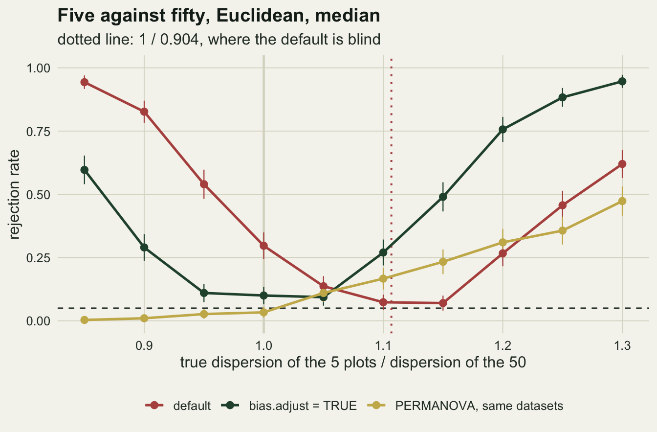
What to report
Give the group sizes next to every dispersion test, and say which centre and which setting of bias.adjust were used. The default is a spatial median with no adjustment, and a methods sentence that says only that betadisper was run leaves a reader unable to tell which test was done.
With unequal groups, set bias.adjust = TRUE and say so. In this grid it brought five against fifty from 0.222 to 0.320 down to 0.060 to 0.102. It did not bring every cell to the nominal level, so in a design like five against fifty an adjusted dispersion p value a little under 0.05 is weaker evidence than it looks, most of all with type = "centroid". The median, which is the default type, left less.
Report the group mean distances with the adjustment applied, and say which group is the more dispersed. Unadjusted, the mean distance of a group of five is shrunk by about 10 per cent relative to a group of fifty, which is a bias in a beta diversity estimate before it is a problem in a test.
Do not reach for permutest() as the fix. In every cell here its rate was within 0.028 of the F test’s.
For the PERMANOVA of Mistake 4: a non-significant betadisper() does not clear an unbalanced PERMANOVA, and once the small group is at least 10 per cent more dispersed the default is the worse of the two checks. With five against fifty the default is at its least sensitive exactly when the small group is somewhat more dispersed, the case Anderson and Walsh flag as the one that makes PERMANOVA too liberal, and even the adjusted test flags a small group that is 10 per cent more dispersed in only 0.270 of datasets; there it let 38 of PERMANOVA’s 50 false rejections through. Report the dispersion test beside the PERMANOVA either way, but do not let its p value carry the argument.
In a balanced design none of this applies. The adjustment is a constant factor there and changes nothing, and no balanced cell was further from 0.05 than 1.8 Monte Carlo standard errors.
Honest limits
Species are independent in all three generators, and there are twenty five of them. Real communities have correlated species and very uneven abundances; the squared-distance closed form does not depend on either, and neither does the design factor by which the adjustment stretches the spread, as long as distances vary about equally within the two groups, but the default spread ratio that factor multiplies depends on how distances vary within a group, and there is no reason it should stay in the range measured here.
Equal true dispersion was produced by drawing both groups from one distribution, so the groups also share a location. With Bray-Curtis and Jaccard a shift in composition changes the dispersion as well, and a null with different locations and equal dispersions is harder to build honestly; it was not attempted.
Only two groups were compared. With three or more groups the F test pools the within-group variance across all of them, and the effect of one small group on that pooled variance is not measured here.
The blind-spot curve and the PERMANOVA beside it use Euclidean distances and a pure change of scale, where “k times more dispersed” has one meaning. For Bray-Curtis or Jaccard there is no single scale factor that does the same, and the curve is not repeated for them.
The permutation tests use 199 permutations per dataset rather than vegan’s 999. More permutations change the resolution of each p value, not the scheme, and the scheme is what carries the bias.
No alternative to the adjustment was measured. What the adjustment leaves comes from scaling the small group’s scatter along with its mean while the pooled standard error follows the large group; no alternative test was run here, so none is recommended. The sqrt.dist and add arguments of betadisper() were left at their defaults. Of the 7524 betadisper() fits in this post, none produced vegan’s warning about negative squared distances being set to zero.
References
Anderson MJ 2006 Biometrics 62(1):245-253 (10.1111/j.1541-0420.2005.00440.x)
Anderson MJ, Ellingsen KE, McArdle BH 2006 Ecology Letters 9(6):683-693 (10.1111/j.1461-0248.2006.00926.x)
Anderson MJ, Walsh DCI 2013 Ecological Monographs 83(4):557-574 (10.1890/12-2010.1)
Stier AC, Geange SW, Hanson KM, Bolker BM 2013 Ecology 94(5):1057-1068 (10.1890/11-1983.1)