library(ggplot2)
library(MASS)
library(vegan)

te_paper  <- "#f5f4ee"
te_ink    <- "#16241d"
te_body   <- "#2c3a31"
te_forest <- "#275139"
te_rust   <- "#b5534e"
te_gold   <- "#c9b458"
te_line   <- "#dad9ca"

theme_datasheet <- function() {
  theme_minimal(base_size = 12) +
    theme(plot.background  = element_rect(fill = te_paper, colour = NA),
          panel.background = element_rect(fill = te_paper, colour = NA),
          panel.grid.major = element_line(colour = te_line, linewidth = 0.3),
          panel.grid.minor = element_blank(),
          text             = element_text(colour = te_body),
          plot.title       = element_text(colour = te_ink, face = "bold"),
          plot.subtitle    = element_text(colour = te_body),
          axis.text        = element_text(colour = te_body))
}Pseudocounts turn read depth into a result
R
vegan
PERMANOVA
microbial ecology
compositional data
ecology tutorial
A fixed 0.5 pseudocount makes a sparse taxon’s log-ratio a function of library size, so unequal sequencing depth is reported as a group effect. Worked in R.
A soil survey sequences the 16S gene in two batches. The first batch went to the machine in March and came back with a median of about seventeen thousand reads per sample; the second went in June, after the facility changed its loading protocol, and came back with about fifty-two thousand. The two batches happen to correspond to the two treatments, because that is how the field season ran. Every analyst in the room knows this is a confound. The question is what to do about it, and the usual answer is a compositional one: divide the depth out on the log scale with a centred log-ratio, which is scale invariant and does not throw away reads. Zeros cannot be logged, so add 0.5 to every count first.
That last sentence is where the trouble is. The detection-limit post showed that a constant substituted at a moving limit turns the laboratory into a trend, and the zeros post said a zero read is such a non-detect; this post is where the two meet the advice of the metabarcoding check: the log-ratio that check ranked at the top reports the sequencer on any taxon sparse enough to have zeros, and the rarefaction it called wasteful is the repair.
The three posts being set against each other are worth naming exactly. Checking a metabarcoding analysis ran this same confounded design, with libraries of seventeen thousand against fifty-two thousand reads, and found that raw counts rejected a true null in 0.973 of runs while rarefied counts, proportions and the centred log-ratio held at 0.060, 0.062 and 0.055, within a Monte Carlo standard error of one another. It recommended dividing by the total, which keeps 0.743 power against the rarefied 0.543, and it concluded that rarefying “is wasteful, and the waste is measurable in power”. Its focal taxon had a share of 0.0006 of the reads, which at those depths is about ten reads a sample and almost never a zero. Compositional analysis and the zero problem showed that the log-ratio of a taxon that was zero tracks whatever value is imputed for it, and named the zero as a value below a detection limit. Values below the detection limit in R showed what happens when that limit moves during a programme: a flat population acquires a decline.
Put those together and the prediction is specific. The detection limit for a sequencing library is of order one read in N, so it moves with depth, and the pseudocount is a constant substituted at it. That should make the log-ratio of any sparse taxon a function of log N, and in a design where depth is confounded with group it should be reported as a group effect. The metabarcoding check did not see this because its focal taxon was not sparse. Most of a real amplicon table is.
This post measures four things. First the size of the bias in closed form, as a function of a taxon’s expected count, which is arithmetic and not simulation. Then the false positive rate of seven analyses on a null taxon as its zero share is swept from 0.03 to 0.90. Then the same bias acting on a whole table at once, through a PERMANOVA on the Aitchison distance under a null grouping, in the regime Weiss and colleagues warned about in 2017, with a measurement of which taxa carry it. Then whether an ordination would have shown the analyst any of this, which turns out to depend on how sparse the table is.
The bias has a closed form, and it is about small counts
Write the centred log-ratio of taxon k in a sample with library size N as the log of its padded count minus the mean of the padded logs. If most taxa in the sample are abundant enough that their counts swamp the pseudocount, that mean is close to log N plus a term that does not depend on N. So the centred log-ratio of one taxon with true share p, at library size N, is approximately the log of pN plus the pseudocount, minus log N, minus a constant.
Take the difference between two groups whose only difference is depth. The constant cancels and what is left is exact arithmetic with no simulation in it:
depth_lo <- 17000
depth_hi <- 52000
pseudo   <- 0.5
ratio_d  <- depth_hi / depth_lo
log_gap  <- log(ratio_d)

clr_shift <- function(mu_lo, ratio, pc) {
  log((ratio * mu_lo + pc) / (mu_lo + pc)) - log(ratio)
}

mu_show   <- c(0, 0.5, 1, 2, 5, 20)
shift_tab <- data.frame(expected_count = mu_show,
                        shift = clr_shift(mu_show, ratio_d, pseudo))
half_at  <- uniroot(function(m) clr_shift(m, ratio_d, pseudo) + 0.5 * log_gap,
                    c(1e-8, 100))$root
tenth_at <- uniroot(function(m) clr_shift(m, ratio_d, pseudo) + 0.1 * log_gap,
                    c(1e-8, 1e4))$root
print(shift_tab, row.names = FALSE, digits = 3)
expected_count shift
0.0 -1.1180
0.5 -0.4103
1.0 -0.2541
2.0 -0.1446
5.0 -0.0631
20.0 -0.0166A taxon that is absent from every sample has a padded count of 0.5 in both groups, so its centred log-ratio differs between the groups by exactly minus the log depth ratio: -1.118 at 17000 against 52000 reads. That endpoint is closed form and owes nothing to any simulation below.
The interesting part is not the endpoint but the approach to it. At an expected count of one read in the shallow library the shift is already -0.254, at two reads -0.145, and at five reads -0.063. Half of the full bias is present at an expected count of 0.29 reads, and a tenth of it survives out to 2.7 reads. The biological noise in the simulations below has a log standard deviation of 0.4, so a shift of a quarter of a log unit is a substantial fraction of one sample’s variation, and it is a shift of the mean, which fifteen samples per group will find.
A zero is the limiting case of a small count, and a count of one or two reads carries part of the same depth-dependent shrinkage. The curve is steep, though: by an expected count of five reads most of the bias has gone. So the taxa that matter are the ones whose expected count is of order one, and in a real table those are the taxa that turn up as zeros somewhere. The community section below tests that directly, by deleting them.
One arithmetic point disposes of an arm before it is simulated. The Bayesian multiplicative replacement that adds 0.5 and renormalises to N plus 0.5 times the number of taxa differs from adding 0.5 alone by a per-sample scale factor, and the centred log-ratio removes per-sample scale factors:
set.seed(4491)
demo_counts <- matrix(rpois(30 * 12, 4), 30, 12)
clr_rows <- function(mat) t(apply(log(mat), 1, function(z) z - mean(z)))
plain_clr <- clr_rows(demo_counts + pseudo)
bayes_clr <- clr_rows((demo_counts + pseudo) /
                        (rowSums(demo_counts) + pseudo * ncol(demo_counts)))
max_gap <- max(abs(plain_clr - bayes_clr))
The two agree to 4.4e-16, which is floating point noise. Any replacement that is a constant plus a per-sample rescaling is the fixed pseudocount wearing a different name, and it inherits every property measured below.
mu_grid <- exp(seq(log(0.001), log(100), length.out = 300))
shift_df <- rbind(
  data.frame(mu = mu_grid, shift = clr_shift(mu_grid, ratio_d, pseudo),
             ratio = sprintf("depth ratio %.1f (17k vs 52k)", ratio_d)),
  data.frame(mu = mu_grid, shift = clr_shift(mu_grid, 10, pseudo),
             ratio = "depth ratio 10 (2k vs 20k)"))

ggplot(shift_df, aes(mu, shift, colour = ratio)) +
  geom_hline(yintercept = c(-log_gap, -log(10)), linetype = "dashed",
             colour = te_body, linewidth = 0.4) +
  geom_vline(xintercept = 1, linetype = "dashed",
             colour = te_body, linewidth = 0.5) +
  geom_line(linewidth = 1) +
  scale_x_log10(breaks = c(0.001, 0.01, 0.1, 1, 10, 100),
                labels = c("0.001", "0.01", "0.1", "1", "10", "100")) +
  scale_colour_manual(values = c(te_rust, te_forest), name = NULL) +
  labs(x = "expected count in the shallow library (reads)",
       y = "shift in the centred log-ratio",
       title = "The pseudocount bites at counts of order one",
       subtitle = "closed form, no simulation; dashed vertical line: one expected read") +
  theme_datasheet() +
  theme(legend.position = "bottom")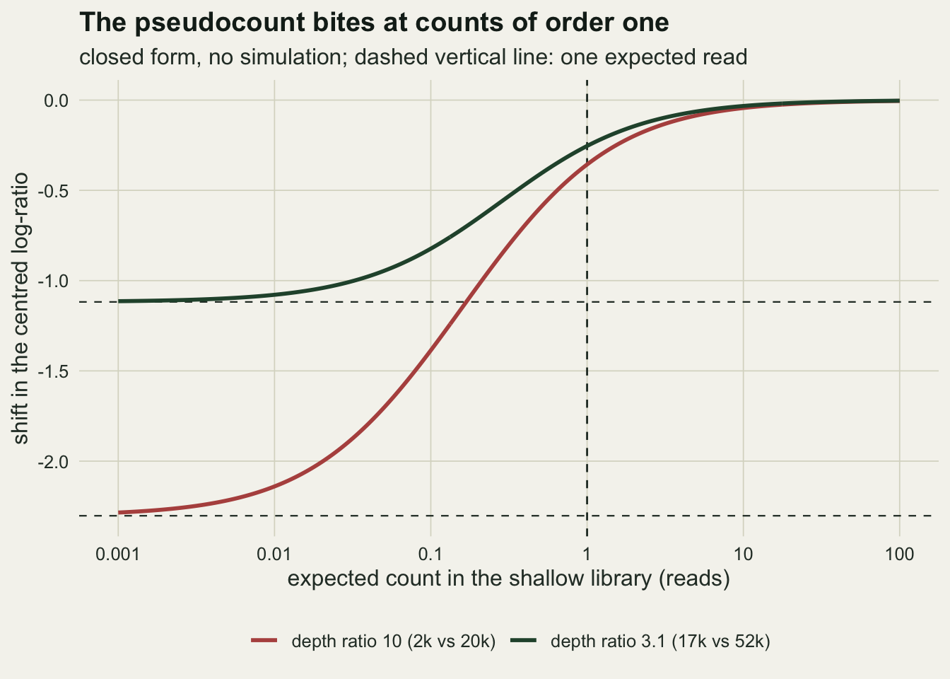
A null taxon, swept from common to nearly absent
The design follows the metabarcoding check so that the comparison is a comparison and not a change of subject: two groups of fifteen samples, multinomial reads, lognormal biological noise on every taxon, and the same two depth regimes, one confounded at 17000 reads against 52000 and one balanced at thirty thousand against thirty thousand. The difference is the focal taxon. Its true share is identical in the two groups in every cell, so every rejection is a false one, and the share is swept across five values so that its zero share runs from almost none to almost all.
n_taxa  <- 40L
n_each  <- 15L
sd_bio  <- 0.4
n_rep   <- 600L
grp_num <- rep(0:1, each = n_each)
grp_fac <- factor(grp_num)
focal   <- 1L
share_grid  <- c(2e-4, 5e-5, 2e-5, 8e-6, 3e-6)
depth_flat  <- 30000
mc_se_rate  <- sqrt(0.05 * 0.95 / n_rep)

set.seed(20260920)
base_share <- exp(rnorm(n_taxa, 0, 1.2))
base_share <- base_share / sum(base_share)

cat("taxa", n_taxa, " samples per group", n_each,
    " biological log sd", sd_bio, "\n")
taxa 40 samples per group 15 biological log sd 0.4 cat("focal shares swept:", format(share_grid, scientific = TRUE), "\n")focal shares swept: 2e-04 5e-05 2e-05 8e-06 3e-06 cat("replicates per cell", n_rep,
" Monte Carlo se at the nominal rate", round(mc_se_rate, 4), "\n")replicates per cell 600 Monte Carlo se at the nominal rate 0.0089 Every constant above was fixed before the first cell ran. The reference community is drawn once, outside the replication loop, so that the five cells differ in the focal taxon’s share and in nothing else; the focal share is set explicitly and the other thirty-nine taxa enter the log-ratio only through the mean of their logs, which is stable from draw to draw. The community section later redraws its base composition in every replicate, because there the composition is the object of study rather than a fixed background.
Seven analyses of that same focal taxon are compared. The first six are applied to the identical table in each replicate. The first is the arm the metabarcoding check ranked at the top under the confound: a centred log-ratio with a fixed 0.5 added, tested with a Welch t test. The second scales the pseudocount with the library, 0.5 times N over the median N, which is the obvious repair and the one a compositional reviewer usually asks for. The third rarefies every library down to the smallest in the run and then takes the same log-ratio; rarefaction here is multinomial resampling with replacement, the usual approximation, rather than subsampling without it. The fourth is a Wilcoxon test on the raw proportions, which needs no pseudocount at all. The fifth is a negative binomial generalised linear model with the log library size as an offset, which puts depth in the model rather than in the data. The sixth is the log of a padded proportion, which is the arm the metabarcoding check actually recommended, written with the same 0.5 and the same denominator convention. The seventh is the two-part test a microbiome statistician asks for when a log-ratio looks bimodal; it runs on its own draws from the same generator, and it shares the section after next with a rank test on the same log-ratio values.
gen_table <- function(share, d_lo, d_hi) {
  lib <- c(rep(d_lo, n_each), rep(d_hi, n_each))
  p_vec <- base_share
  p_vec[focal] <- share
  p_vec <- p_vec / sum(p_vec)
  cnt <- matrix(0L, 2 * n_each, n_taxa)
  for (i in seq_len(2 * n_each)) {
    q_i <- p_vec * exp(rnorm(n_taxa, 0, sd_bio))
    cnt[i, ] <- as.integer(rmultinom(1, lib[i], q_i / sum(q_i)))
  }
  list(cnt = cnt, lib = lib)
}

clr_focal <- function(cnt, pc) {
  lg <- log(cnt + pc)
  lg[, focal] - rowMeans(lg)
}
welch_p <- function(y) t.test(y[grp_num == 0], y[grp_num == 1])$p.value
rarefy_rows <- function(cnt, depth) {
  t(apply(cnt, 1, function(r_i) rmultinom(1, depth, r_i / sum(r_i))[, 1]))
}

one_rep <- function(share, d_lo, d_hi) {
  tab <- gen_table(share, d_lo, d_hi)
  cnt <- tab$cnt
  lib <- tab$lib
  prop <- cnt[, focal] / lib
  cl_fix <- clr_focal(cnt, pseudo)
  c(zero_share = mean(cnt[, focal] == 0),
    clr_fixed  = welch_p(cl_fix),
    clr_scaled = welch_p(clr_focal(cnt, pseudo * lib / median(lib))),
    clr_rarefy = welch_p(clr_focal(rarefy_rows(cnt, min(lib)), pseudo)),
    wilcox_prop = suppressWarnings(
      wilcox.test(prop[grp_num == 0], prop[grp_num == 1])$p.value),
    nb_offset = tryCatch(suppressWarnings(
      summary(glm.nb(cnt[, focal] ~ grp_num + offset(log(lib))))
      )$coefficients["grp_num", 4], error = function(e) NA_real_),
    clr_rank = suppressWarnings(
      wilcox.test(cl_fix[grp_num == 0], cl_fix[grp_num == 1])$p.value),
    prop_pad = tryCatch(welch_p(log((cnt[, focal] + pseudo) /
                                      (lib + pseudo * n_taxa))),
                        error = function(e) NA_real_))
}

run_cell <- function(share, d_lo, d_hi) {
  mat <- t(replicate(n_rep, one_rep(share, d_lo, d_hi)))
  out <- c(zero_share = mean(mat[, "zero_share"]),
           colMeans(mat[, -1] < 0.05, na.rm = TRUE))
  c(out, usable_wilcox = sum(!is.na(mat[, "wilcox_prop"])),
    usable_nb = sum(!is.na(mat[, "nb_offset"])),
    usable_pad = sum(!is.na(mat[, "prop_pad"])))
}

set.seed(7731)
res_conf <- t(vapply(share_grid, function(s) run_cell(s, depth_lo, depth_hi),
                     numeric(11)))
res_flat <- t(vapply(share_grid, function(s) run_cell(s, depth_flat, depth_flat),
                     numeric(11)))
rate_conf <- as.data.frame(res_conf)
rate_flat <- as.data.frame(res_flat)
rate_conf$share <- share_grid
rate_flat$share <- share_grid
z_nominal <- function(r) (r - 0.05) / mc_se_rate
show_cols  <- c("clr_fixed", "clr_scaled", "clr_rarefy", "wilcox_prop",
                "nb_offset")
hold_max <- max(c(rate_conf$clr_rarefy, rate_conf$nb_offset))
nb_min   <- min(rate_conf$nb_offset)
rar_min  <- min(rate_conf$clr_rarefy)
scaled_max <- max(rate_conf$clr_scaled)
flat_max <- max(rate_flat[, show_cols])
pad_gap  <- max(abs(rate_conf$prop_pad - rate_conf$clr_fixed))
wilcox_unusable <- n_rep - rate_conf$usable_wilcox[5]
nb_unusable <- n_rep - rate_conf$usable_nb[5]
pad_unusable <- n_rep - rate_conf$usable_pad[5]
print(round(rate_conf[, c("zero_share", show_cols, "prop_pad")], 3),
      row.names = FALSE)
zero_share clr_fixed clr_scaled clr_rarefy wilcox_prop nb_offset prop_pad
0.025 0.062 0.047 0.055 0.047 0.063 0.060
0.259 0.102 0.140 0.048 0.070 0.057 0.092
0.521 0.588 0.135 0.040 0.142 0.038 0.597
0.755 0.980 0.127 0.028 0.193 0.032 0.987
0.894 1.000 0.050 0.013 0.075 0.007 1.000print(round(rate_flat[, c("zero_share", show_cols)], 3), row.names = FALSE) zero_share clr_fixed clr_scaled clr_rarefy wilcox_prop nb_offset
0.009 0.047 0.047 0.050 0.045 0.075
0.233 0.038 0.038 0.040 0.037 0.060
0.538 0.055 0.055 0.043 0.052 0.047
0.774 0.040 0.040 0.027 0.047 0.012
0.905 0.028 0.028 0.015 0.019 0.000cat("negative binomial fits that converged, per cell, of", n_rep, ":",
rate_conf$usable_nb, "\n")negative binomial fits that converged, per cell, of 600 : 600 600 600 600 583 The five cells of the confounded regime put the focal taxon’s zero share at 0.03, 0.26, 0.52, 0.76, 0.89. The fixed pseudocount log-ratio rejects a true null in 0.062 of tables at the first of those, which reproduces the metabarcoding check’s verdict, and then in 0.102, 0.588, 0.980 and 1.000 as the taxon gets sparser, against a Monte Carlo standard error of 0.0089 at the nominal rate. At the sparsest cell the test rejects every table it is given.
At balanced depth the same analysis on the same generator rejects in 0.047, 0.038, 0.055, 0.040, 0.028 across the same five focal shares. The design constant across the two panels is the share, not the zero share: at equal depth the focal taxon is absent in 0.01, 0.23, 0.54, 0.77, 0.90 of samples, which differs from the confounded panel most at the first cell. The pseudocount is not the problem on its own; the pseudocount with a depth difference is.
The repairs separate cleanly, and they miss in the other direction. Rarefying to the smallest library first and then taking the identical log-ratio gives 0.055, 0.048, 0.040, 0.028, 0.013 in the confounded regime, and the negative binomial model with a log depth offset gives 0.063, 0.057, 0.038, 0.032, 0.007. Neither leaks: across those ten confounded-regime rates the highest either of them reaches is 0.063, 1.5 Monte Carlo standard errors above the nominal rate. Both go conservative as the taxon empties, and the count model goes furthest: its lowest cell is 0.007, 4.8 standard errors below nominal, against the rarefied 0.013 at 4.1 below. At the sparsest cell the negative binomial fit also failed to converge in 17 of 600 replicates, and that cell’s rate is computed on the rest.
Scaling the pseudocount with the library is a different matter: it peaks at 0.140 at a zero share of 0.26, 10.1 standard errors above nominal, and it is above nominal in every cell but the first. The reason is visible in the design: scaling the pseudocount equalises what is added to a zero relative to depth, but the two groups do not have the same number of zeros to begin with, so the correction is applied to different fractions of each group.
The Wilcoxon test on proportions, which never touches a pseudocount, reaches 0.193 at its worst cell. Its failure is a different one: ties. A proportion of exactly zero occurs in both groups, but at unequal depth the non-zero proportions have different granularity, so the rank structure carries depth. At the sparsest cell the test is undefined in 17 of 600 replicates, where the taxon was absent from every sample in the table.
The arm the metabarcoding check recommended does not escape either, once a zero forces a pseudocount back into it. The log of a padded proportion, the log of x plus 0.5 over N plus 0.5 times the number of taxa, tested with the same Welch test, rejects in 0.060, 0.092, 0.597, 0.987, 1.000. The largest difference between that curve and the centred log-ratio curve anywhere in the sweep is 0.010, or 1.1 Monte Carlo standard errors, so the two are the same curve for practical purposes and the padded proportion is left out of the figure below to avoid drawing one line on top of another. Like the Wilcoxon test, it is undefined in 17 of 600 replicates at the sparsest cell: where the taxon is absent from the whole table the padded proportion takes one constant value in each group, and the two constants differ by exactly the log depth ratio, which is the closed form of the first section arriving without a test to report it. Centring is not what breaks. The constant added under the log is.
meth_key <- c(clr_fixed = "CLR, fixed 0.5",
              clr_scaled = "CLR, depth-scaled 0.5",
              clr_rarefy = "rarefy, then CLR",
              wilcox_prop = "Wilcoxon on proportions",
              nb_offset = "NB GLM, log-depth offset")
long_rates <- function(tab, lab) {
  do.call(rbind, lapply(names(meth_key), function(m) {
    data.frame(zero_share = tab$zero_share, rate = tab[[m]],
               method = meth_key[[m]], regime = lab)
  }))
}
rates_df <- rbind(
  long_rates(rate_conf, sprintf("%d vs %d reads", depth_lo, depth_hi)),
  long_rates(rate_flat, sprintf("%d vs %d reads", depth_flat, depth_flat)))
rates_df$method <- factor(rates_df$method, levels = unname(meth_key))

ggplot(rates_df, aes(zero_share, rate, colour = method)) +
  geom_hline(yintercept = 0.05, linetype = "dashed",
             colour = te_body, linewidth = 0.5) +
  geom_line(linewidth = 0.9) +
  geom_point(size = 1.8) +
  facet_wrap(~regime) +
  scale_colour_manual(values = c(te_rust, te_gold, te_forest,
                                 "#8d8b78", te_ink), name = NULL) +
  scale_y_continuous(limits = c(0, 1)) +
  labs(x = "zero share of the focal taxon", y = "false positive rate at 0.05",
       title = "Only rarefying and the count model hold their rate",
       subtitle = "the focal taxon's true share is identical in both groups in every cell") +
  theme_datasheet() +
  theme(legend.position = "bottom") +
  guides(colour = guide_legend(nrow = 2))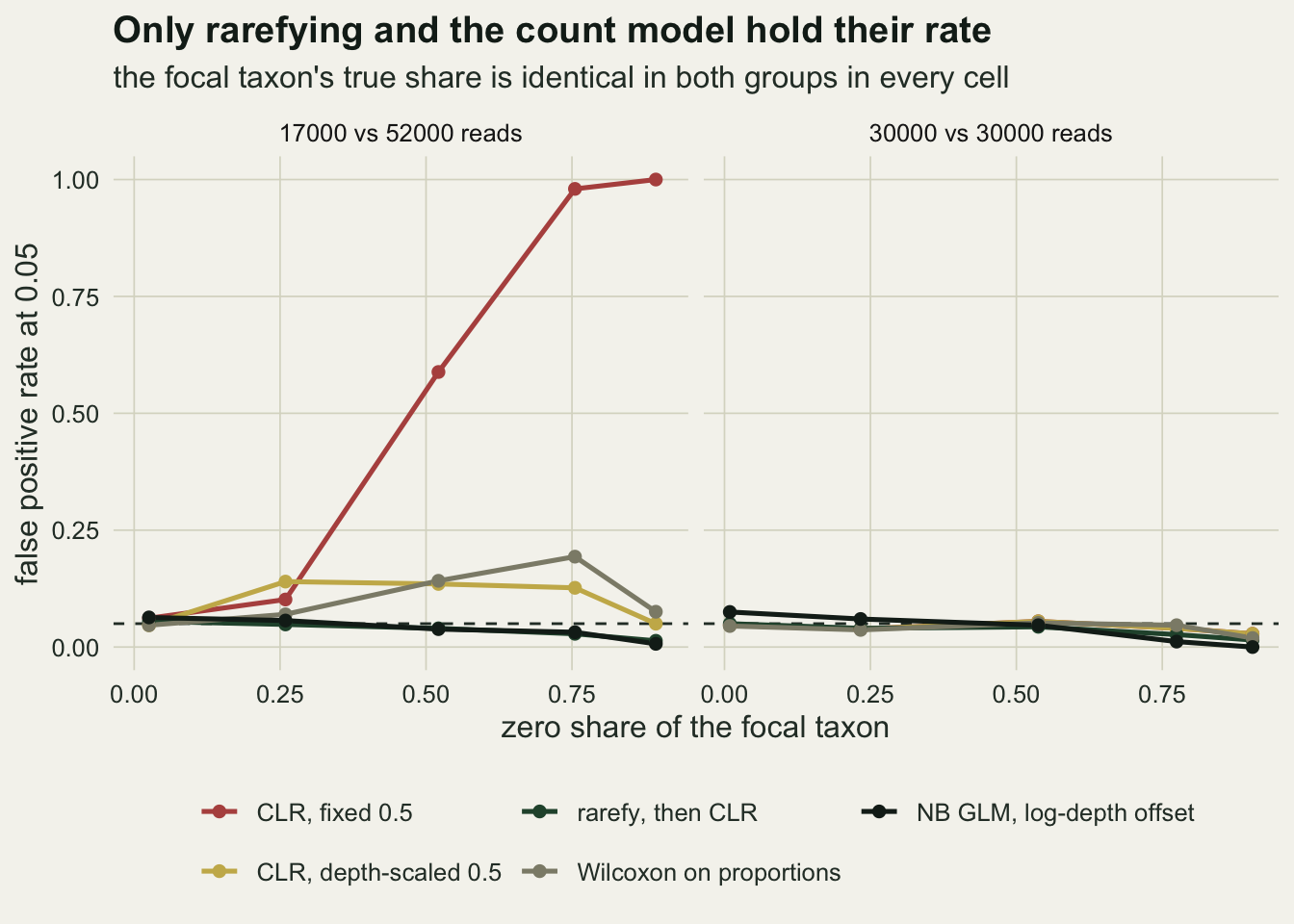
The test is not the problem, and a zero-aware test is worse
A reasonable objection is that the failure is the Welch test rather than the pseudocount. A centred log-ratio on a sparse taxon is bimodal: the zero samples pile up at the padded value and the rest sit above it, and a t test on such a thing has no business being trusted. Two checks settle this. The first applies a Wilcoxon rank sum test to the identical log-ratio values. The second is the two-part test that is usually proposed for zero-inflated compositions: a Fisher exact test on presence and absence by group, a Welch test on the log-ratio among the samples where the taxon was seen, and Fisher’s method to combine the two.
two_part_p <- function(cnt, lib) {
  x_focal <- cnt[, focal]
  present <- x_focal > 0
  p_pres <- tryCatch(
    fisher.test(table(factor(present, c(FALSE, TRUE)), grp_num))$p.value,
    error = function(e) NA_real_)
  cl_val <- clr_focal(cnt, pseudo)
  keep <- present & is.finite(cl_val)
  p_pos <- if (sum(keep & grp_num == 0) >= 2 && sum(keep & grp_num == 1) >= 2) {
    tryCatch(t.test(cl_val[keep & grp_num == 0],
                    cl_val[keep & grp_num == 1])$p.value,
             error = function(e) NA_real_)
  } else NA_real_
  p_both <- c(p_pres, p_pos)
  p_both <- p_both[!is.na(p_both)]
  if (!length(p_both)) return(NA_real_)
  pchisq(-2 * sum(log(p_both)), df = 2 * length(p_both), lower.tail = FALSE)
}

set.seed(5518)
two_part_rate <- vapply(share_grid, function(s) {
  p_vals <- replicate(n_rep, {
    tab <- gen_table(s, depth_lo, depth_hi)
    two_part_p(tab$cnt, tab$lib)
  })
  mean(p_vals < 0.05, na.rm = TRUE)
}, numeric(1))
gap_cell <- which.max(two_part_rate - rate_conf$clr_fixed)
form_tab <- data.frame(zero_share = round(rate_conf$zero_share, 2),
                       clr_welch = rate_conf$clr_fixed,
                       clr_wilcoxon = rate_conf$clr_rank,
                       two_part = two_part_rate)
print(round(form_tab, 3), row.names = FALSE)
zero_share clr_welch clr_wilcoxon two_part
0.03 0.062 0.057 0.023
0.26 0.102 0.088 0.915
0.52 0.588 0.375 0.977
0.76 0.980 0.912 0.647
0.89 1.000 0.998 0.092The rank test on the same log-ratio values rejects in 0.057, 0.088, 0.375, 0.912, 0.998 across the sweep. It is a little better than the Welch test in the middle of the range and just as bad at the end. The failure is in the values, not in the test applied to them.
The two-part test is worse than either. On independently drawn tables from the same generator it rejects in 0.023, 0.915, 0.977, 0.647, 0.092, reaching 0.977 at a zero share of 0.52. The widest gap is at a zero share of 0.26, where the two-part test rejects 0.915 of tables and the plain Welch test on the same log-ratio rejects 0.102 on its own tables. Making the test zero-aware makes it depth-aware in the wrong direction, because whether a rare taxon is detected at all is the most depth-dependent thing about it: a deeper library sees it more often, so the presence part of the test reads the sequencer directly. The combination rule works against that, if anything: Fisher’s method assumes uniform p values, and a Fisher exact p on a two by two presence table is discrete and conservative, so the excess above happens in spite of the combination and not because of it. The rate falls again at the sparsest cell only because there the taxon is nearly absent everywhere and the Fisher table stops discriminating.
The same bias moves a whole community
The single-taxon result is the easy one to argue away: analysts do not test one taxon, they run a PERMANOVA. Weiss and colleagues warned in 2017 that normalisations other than rarefying are vulnerable to artefacts from library size, and reported that for groups differing about tenfold in average library size rarefying lowers the false discovery rate of a differential abundance analysis. They did not test a log-ratio distance under a null grouping, and their normalisation set was rarefying against DESeq-type and cumulative-sum scaling rather than the centred log-ratio. This section is an extension of that warning to the arrangement an ecologist is most likely to run, in the simplest form that shows it. There is no group effect at all in the generator: the two groups are drawn from the same community, and the only thing that differs is the library size.
The base composition is redrawn in every replicate, so the rejection rate is an average over communities rather than a property of one lucky draw. Five analyses run on each table: the Aitchison distance, which is Euclidean distance on the centred log-ratio with a fixed 0.5, Bray-Curtis on proportions, both of those again after rarefying to the smallest library, and the Aitchison distance once more on only those taxa that have no zero anywhere in the table. The last one is the arm that says where the effect lives, and the code also keeps the number of taxa it had to delete.
n_taxa2 <- 60L
n_rep2  <- 120L
n_perm  <- 199L
depth_pairs <- list(c(20000, 20000), c(5000, 20000), c(2000, 20000),
                    c(1000, 20000), c(500, 20000))

gen_table2 <- function(d_lo, d_hi) {
  b_vec <- exp(rnorm(n_taxa2, 0, 1.5))
  b_vec <- b_vec / sum(b_vec)
  lib <- c(rep(d_lo, n_each), rep(d_hi, n_each))
  cnt <- matrix(0L, 2 * n_each, n_taxa2)
  for (i in seq_len(2 * n_each)) {
    q_i <- b_vec * exp(rnorm(n_taxa2, 0, sd_bio))
    cnt[i, ] <- as.integer(rmultinom(1, lib[i], q_i / sum(q_i)))
  }
  list(cnt = cnt, lib = lib)
}
aitchison <- function(cnt) dist(clr_rows(cnt + pseudo))

one_rep2 <- function(d_lo, d_hi) {
  tab <- gen_table2(d_lo, d_hi)
  cnt <- tab$cnt
  cnt_r <- rarefy_rows(cnt, min(tab$lib))
  d_ait <- aitchison(cnt)
  complete <- apply(cnt, 2, min) > 0
  c(aitchison = adonis2(d_ait ~ grp_fac, permutations = n_perm)$`Pr(>F)`[1],
    bray = adonis2(vegdist(cnt / rowSums(cnt), "bray") ~ grp_fac,
                   permutations = n_perm)$`Pr(>F)`[1],
    aitchison_rar = adonis2(aitchison(cnt_r) ~ grp_fac,
                            permutations = n_perm)$`Pr(>F)`[1],
    bray_rar = adonis2(vegdist(cnt_r / rowSums(cnt_r), "bray") ~ grp_fac,
                       permutations = n_perm)$`Pr(>F)`[1],
    dispersion = permutest(betadisper(d_ait, grp_fac),
                           permutations = n_perm)$tab$`Pr(>F)`[1],
    aitchison_nz = if (sum(complete) >= 3) {
      adonis2(aitchison(cnt[, complete, drop = FALSE]) ~ grp_fac,
              permutations = n_perm)$`Pr(>F)`[1]
    } else NA_real_,
    taxa_with_zero = sum(!complete),
    min_kept = if (any(complete)) {
      median(apply(cnt[, complete, drop = FALSE], 2, min))
    } else NA_real_,
    zero_share = mean(cnt == 0))
}

set.seed(9081)
act_two <- as.data.frame(t(vapply(depth_pairs, function(dp) {
  mat <- t(replicate(n_rep2, one_rep2(dp[1], dp[2])))
  c(depth_lo = dp[1], ratio = dp[2] / dp[1],
    zero_share = mean(mat[, "zero_share"]),
    taxa_with_zero = median(mat[, "taxa_with_zero"]),
    min_kept = median(mat[, "min_kept"], na.rm = TRUE),
    colMeans(mat[, 1:5] < 0.05),
    aitchison_nz = mean(mat[, "aitchison_nz"] < 0.05, na.rm = TRUE))
}, numeric(11))))
mc_se2 <- sqrt(0.25 / n_rep2)
mc_se2_nom <- sqrt(0.05 * 0.95 / n_rep2)
print(round(act_two, 3), row.names = FALSE)
depth_lo ratio zero_share taxa_with_zero min_kept aitchison bray
20000 1 0.002 1 48.5 0.075 0.058
5000 4 0.011 6 14.0 0.167 0.033
2000 10 0.036 15 7.0 0.633 0.067
1000 20 0.062 24 4.5 0.900 0.042
500 40 0.112 35 3.0 1.000 0.150
aitchison_rar bray_rar dispersion aitchison_nz
0.058 0.067 0.075 0.058
0.083 0.058 0.867 0.083
0.042 0.058 1.000 0.125
0.025 0.033 1.000 0.100
0.033 0.033 1.000 0.117With both groups at twenty thousand reads the Aitchison PERMANOVA rejects the null grouping in 0.075 of tables, which is consistent with the nominal rate. Shorten one group’s libraries and it climbs: 0.167 at a fourfold depth difference, 0.633 at tenfold, 0.900 at twentyfold, and 1.000 at fortyfold, with a Monte Carlo standard error of at most 0.046. Bray-Curtis on proportions is far better behaved but not clean: it runs from 0.033 to 0.150, and its worst cell is 5.0 standard errors above nominal on the standard error of 0.020 that applies at the nominal rate. Rarefying to the smallest library first holds both distances down: the highest rate reached by the rarefied Aitchison distance anywhere on the grid is 0.083 and by rarefied Bray-Curtis 0.067.
Which taxa carry it is a separate question from how many cells are zero, and the two counts give opposite impressions. At the tenfold contrast, where the Aitchison test rejects 63 per cent of null groupings, only 3.6 per cent of the cells in the table are zero, which sounds like far too few to matter. The zeros are not spread evenly over the table. They sit in a median of 15 of the 60 taxa, 25 per cent of them. Delete exactly those taxa, keep the ones observed in every sample, and the Aitchison test on what is left rejects in 0.125 of tables instead of 0.633. The same deletion takes the fortyfold contrast from 1.000 to 0.117.
So it is the taxa that touch the pseudocount, and not the general mass of small counts, that carry this. The survivors are not an abundant subset either: at the tenfold contrast the median retained taxon’s smallest count anywhere in the table is 7 reads. The closed form of the first section puts that taxon’s depth shift at -0.062 of a log unit, against -2.303 for a cell that is zero, which is the whole of the difference. The share of cells is the wrong denominator for the question, because Euclidean distance adds up whole taxa, and a taxon that is zero in some of the shallow libraries is displaced along its own axis in every sample it has.
The dispersion test tells the same story in the vocabulary of four common PERMANOVA mistakes. Betadisper on the Aitchison distance rejects in 0.075 of runs at equal depth and 1.000 at tenfold, so the shallow group is genuinely more spread out on this distance as well as displaced. Anderson and Walsh set out in 2013 why a PERMANOVA on groups with unequal dispersion is not testing what its user thinks; here the unequal dispersion is manufactured by the pseudocount and the depth together, and a reader who checks betadisper and finds it significant will at least know not to call the result a location difference.
perm_key <- c(aitchison = "Aitchison (CLR, fixed 0.5)",
              aitchison_nz = "Aitchison, zero-free taxa only",
              bray = "Bray-Curtis on proportions",
              aitchison_rar = "rarefy, then Aitchison",
              dispersion = "betadisper on Aitchison")
perm_df <- do.call(rbind, lapply(names(perm_key), function(m) {
  data.frame(ratio = act_two$ratio, rate = act_two[[m]], test = perm_key[[m]])
}))
perm_df$test <- factor(perm_df$test, levels = unname(perm_key))

ggplot(perm_df, aes(ratio, rate, colour = test)) +
  geom_hline(yintercept = 0.05, linetype = "dashed",
             colour = te_body, linewidth = 0.5) +
  geom_line(linewidth = 0.9) +
  geom_point(size = 2) +
  scale_x_log10(breaks = act_two$ratio,
                labels = sprintf("%.0f", act_two$ratio)) +
  scale_y_continuous(limits = c(0, 1)) +
  scale_colour_manual(values = c(te_rust, te_ink, te_forest, "#8d8b78",
                                 te_gold), name = NULL) +
  labs(x = "ratio of the two groups' library sizes",
       y = "rejection rate under a null grouping",
       title = "A depth contrast read as a community difference",
       subtitle = "no group effect exists in the generator at any point on these curves") +
  theme_datasheet() +
  theme(legend.position = "bottom") +
  guides(colour = guide_legend(nrow = 3))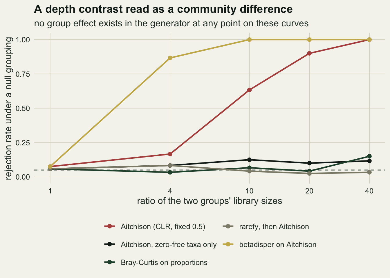
Whether an ordination shows it depends on the sparsity
A natural defence is that this would be visible in an ordination: run a principal component analysis on the centred log-ratio matrix and the depth gradient will be the first axis, so anyone who looks at the picture will see the problem. That is a claim about a population of tables and not about one, so one table cannot settle it. The arrangement here is forty samples with no groups at all, library sizes spread smoothly from one thousand to forty thousand reads, and three settings that change how sparse the table is: sixty taxa with a moderate spread of abundances, two hundred taxa with the same spread, and two hundred with a wider one. Each draw gets a fresh community. For each draw the code regresses each of the first six principal components on log library size and keeps the r squared.
n_grad   <- 200L
n_grad_ad <- 120L
n_samp3  <- 40L
lib3     <- round(exp(seq(log(1000), log(40000), length.out = n_samp3)))
log_lib  <- log(lib3)
grad_set <- list(c(60, 1.5), c(200, 1.5), c(200, 2.5))
grad_lab <- c("60 taxa, spread 1.5", "200 taxa, spread 1.5",
              "200 taxa, spread 2.5")

gen_grad <- function(n_tx, sd_base) {
  b_vec <- exp(rnorm(n_tx, 0, sd_base))
  b_vec <- b_vec / sum(b_vec)
  cnt <- matrix(0L, n_samp3, n_tx)
  for (i in seq_len(n_samp3)) {
    q_i <- b_vec * exp(rnorm(n_tx, 0, sd_bio))
    cnt[i, ] <- as.integer(rmultinom(1, lib3[i], q_i / sum(q_i)))
  }
  cnt
}
depth_r2 <- function(cnt) {
  sc <- prcomp(clr_rows(cnt + pseudo))$x[, 1:6]
  apply(sc, 2, function(z) summary(lm(z ~ log_lib))$r.squared)
}

set.seed(771)
grad_raw <- lapply(grad_set, function(g) t(replicate(n_grad, {
  cnt <- gen_grad(as.integer(g[1]), g[2])
  c(depth_r2(cnt), zero = mean(cnt == 0))
})))
names(grad_raw) <- grad_lab
grad_sum <- data.frame(
  zeros   = vapply(grad_raw, function(m) median(m[, "zero"]), numeric(1)),
  pc1_med = vapply(grad_raw, function(m) median(m[, 1]), numeric(1)),
  pc1_q25 = vapply(grad_raw, function(m) unname(quantile(m[, 1], 0.25)),
                   numeric(1)),
  pc1_q75 = vapply(grad_raw, function(m) unname(quantile(m[, 1], 0.75)),
                   numeric(1)),
  pc1_best = vapply(grad_raw,
                    function(m) mean(apply(m[, 1:6], 1, which.max) == 1),
                    numeric(1)))
print(round(grad_sum, 3))
zeros pc1_med pc1_q25 pc1_q75 pc1_best
60 taxa, spread 1.5 0.030 0.159 0.047 0.339 0.6
200 taxa, spread 1.5 0.101 0.833 0.786 0.865 1.0
200 taxa, spread 2.5 0.361 0.978 0.971 0.983 1.0set.seed(3324)
grad_ad <- t(replicate(n_grad_ad, {
cnt <- gen_grad(60L, 1.5)
cnt_r <- rarefy_rows(cnt, min(lib3))
c(aitchison = adonis2(aitchison(cnt) ~ log_lib,
permutations = n_perm)$`Pr(>F)`[1],
bray = adonis2(vegdist(cnt / rowSums(cnt), "bray") ~ log_lib,
permutations = n_perm)$`Pr(>F)`[1],
rarefied = adonis2(aitchison(cnt_r) ~ log_lib,
permutations = n_perm)$`Pr(>F)`[1])
}))
grad_rate <- colMeans(grad_ad < 0.05)
mc_se_ad <- sqrt(0.05 * 0.95 / n_grad_ad)
cat("gradient PERMANOVA rejection at 0.05:", round(grad_rate, 3), "\n")gradient PERMANOVA rejection at 0.05: 0.683 0.075 0.1 The answer depends entirely on how sparse the table is, and not in the direction that would be comfortable. On the sixty-taxon setting, the one act two used and the least sparse of the three at 3.0 per cent zero cells, log library size explains a median of 0.159 of the variance in PC1, with the middle half of the draws between 0.047 and 0.339, and PC1 is the component most strongly related to depth in 120 of the 200 draws. Raise the richness to two hundred taxa and the zero share goes to 10.1 per cent, log depth explains a median 0.833 of PC1, and PC1 is the depth axis in 200 of 200 draws. Widen the abundance spread as well, to 36.1 per cent zeros, and the median rises to 0.978.
A real 16S table has hundreds to thousands of amplicon variants and is mostly zeros, so it sits at the sparse end of that range, and there the first axis of a log-ratio ordination is largely a picture of library size. An analyst who reads that axis as community structure is reading the sequencer, and that is the more common hazard. The comfortable version of the claim, that the depth gradient would announce itself on PC1 and so could not be missed, is the one that fails: it fails exactly where the table is nearly complete, and there the artefact does not go away, it stops dominating the first axis.
grad_long <- do.call(rbind, lapply(seq_along(grad_raw), function(j) {
  m <- grad_raw[[j]]
  data.frame(
    regime = sprintf("%s\n%.0f per cent zeros", grad_lab[j],
                     100 * median(m[, "zero"])),
    pc = factor(rep(1:6, each = nrow(m))),
    r2 = as.vector(m[, 1:6]))
}))
grad_long$regime <- factor(grad_long$regime, levels = unique(grad_long$regime))
grad_long$first <- ifelse(grad_long$pc == "1", "PC1", "later")

ggplot(grad_long, aes(pc, r2, fill = first)) +
  geom_boxplot(colour = te_ink, linewidth = 0.35, outlier.size = 0.5,
               outlier.colour = te_body) +
  facet_wrap(~regime, nrow = 1) +
  scale_fill_manual(values = c(PC1 = te_rust, later = te_line),
                    guide = "none") +
  scale_y_continuous(limits = c(0, 1)) +
  labs(x = "principal component of the CLR matrix",
       y = "r squared against log library size",
       title = "Sparsity decides whether depth lands on the first axis",
       subtitle = sprintf("%d draws per panel; forty samples, no groups, depth from 1k to 40k reads", n_grad)) +
  theme_datasheet()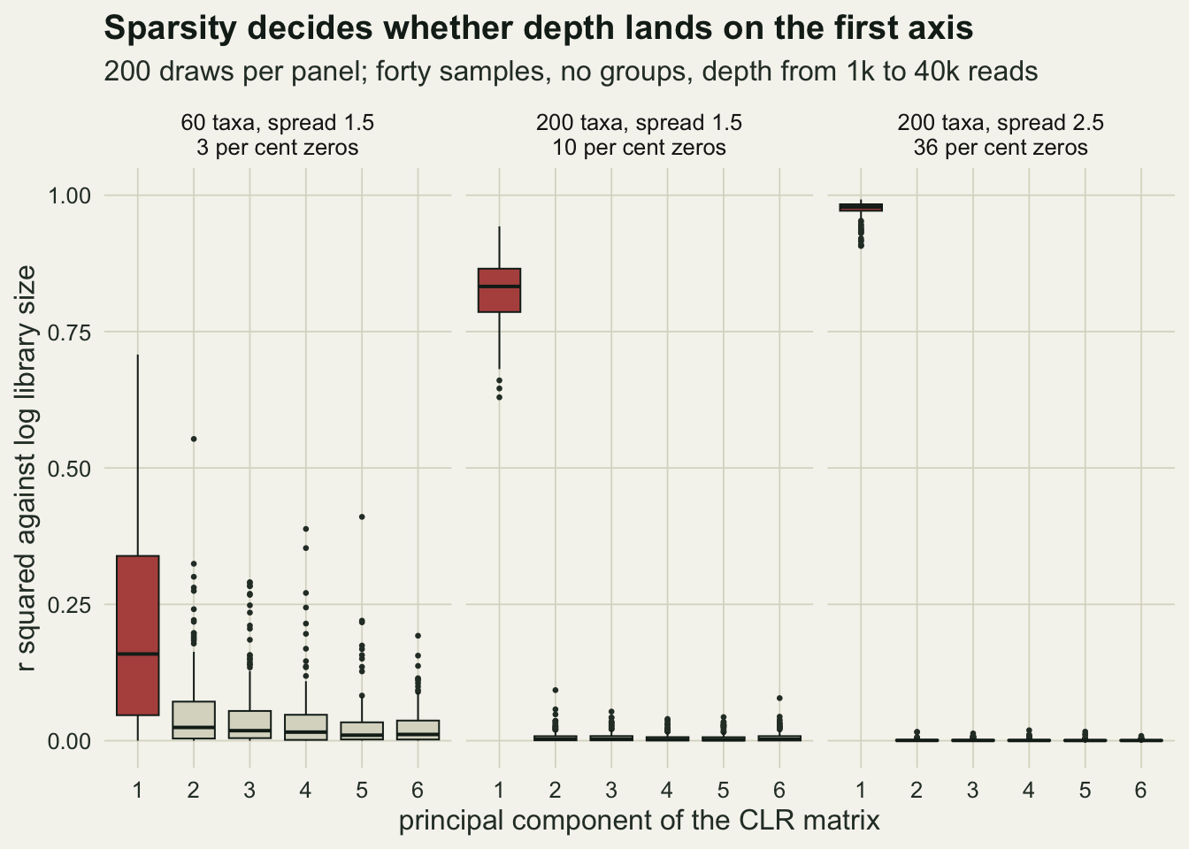
The test that names depth as a predictor finds it either way. On the sixty-taxon setting, a PERMANOVA with log library size as a continuous predictor rejects in 0.683 of draws on the Aitchison distance, against 0.075 on Bray-Curtis on proportions and 0.100 after rarefying, over 120 draws with a standard error of 0.020 at the nominal rate. That is the regime where the picture would not have warned anyone: in half the draws log depth accounts for less than 0.159 of PC1, and the p value finds the shift anyway. So an ordination is evidence when it does show a depth gradient and is not evidence when it does not.
What to report
Give the zero share of every taxon you make a claim about, next to the claim. The false positive rate of the fixed-pseudocount log-ratio was 0.062 at a zero share of 0.03 and 0.980 at a zero share of 0.76, on the same generator, the same depths and the same test. One number separates a trustworthy result from a certainty of the wrong kind, and it costs nothing to print.
Report the library sizes by group, and report them as a distribution, not a mean. A threefold difference in median depth between two treatments is enough for everything above. If the depths are balanced, say so: at equal depth the highest rate any of the five analyses in the figure reached, at any sparsity, was 0.075.
Say which pseudocount was used and whether it is a constant. If it is, the claim about any sparse taxon is partly a claim about that constant, which is the point the zero problem makes in general. Adding 0.5 and renormalising is the same thing under a log-ratio, to 4.4e-16, so the Bayesian label does not buy anything here.
For a differential abundance question on a sparse taxon under unequal depth, report the count model, and report where it is conservative. The negative binomial fit with an offset of log library size never leaked: 0.063, 0.057, 0.038, 0.032, 0.007 across the sweep. Its highest rate is 1.5 Monte Carlo standard errors above nominal and its lowest is 4.8 below, so on the sparsest taxa it is conservative rather than valid, and it loses power there accordingly. It does not discard reads, and depth belongs in the model. If a distance-based community test is the question instead, rarefy: on the Aitchison distance at a tenfold depth contrast the null grouping was rejected in 0.633 of tables without rarefying and 0.042 with it.
Run betadisper whenever the distance is an Aitchison distance and the depths are unequal. It rejected in 1.000 of the tenfold-contrast tables here, and a significant dispersion test is the cheapest available warning that a location claim is not safe.
Honest limits
The repair is not symmetric with the problem. Rarefying protects the error rate and costs power, exactly as checking a metabarcoding analysis measured on a taxon that had no zeros, and nothing above measures that cost at these sparsities. The power cost is the whole of the case McMurdie and Holmes made against rarefying in 2014, on the ground that discarding reads is statistically inefficient; this post does not dispute it, it bounds where it applies. Rarefaction is implemented here as multinomial resampling with replacement rather than subsampling without it, which is the usual approximation and adds a little variance to the shallow group’s own counts. The honest reading of the two posts together is that the ranking depends on the zero share: where a taxon is well observed the log-ratio is both valid and more powerful, and where it is sparse the log-ratio is invalid and the comparison of power does not arise. No single rule covers a whole table, and a table has taxa of both kinds in it.
The library sizes within a group are fixed here, not drawn. That makes the closed-form endpoint exact and the simulation clean, and it is not how a run comes off a machine: the metabarcoding check used a lognormal library size with a log standard deviation of 0.55 around each group’s median, which is more realistic. How much within-group spread in depth dilutes the contrast at a given median ratio is not measured here, and should not be assumed large.
Whether a threefold median depth difference between batches is typical is a question about laboratories, not about statistics, and this post cannot answer it. It is the value the earlier post used and it was kept so that the two are comparable. The act two curve is the better guide to the general shape: the rejection rate under a null grouping was 0.167 at a fourfold ratio and 1.000 at fortyfold, so the artefact grows smoothly with the depth ratio rather than appearing suddenly at one value.
Every table here is multinomial with lognormal biological noise and no overdispersion beyond that, no compositional group effect, and no correlation structure among taxa. Real amplicon data have all three. The negative binomial model was fitted to data that a negative binomial does not exactly describe, and it held its rate anyway; that is reassuring rather than conclusive, and a model-based analysis should be checked against its own residuals rather than trusted because it worked in a simulation with a different generator.
The two-part test measured here is one specific construction, Fisher exact on presence plus a Welch test on the observed log-ratios, combined by Fisher’s method. A hurdle model that puts log depth into the presence part as well would not fail the way this one does, because the depth dependence of detection would then be modelled rather than tested. The result above should be read as a warning about the naive two-part test, not as a claim that no zero-aware method can work.
The act two generator has no group effect at all, so everything reported there is a false positive rate and nothing is a power comparison. A rarefied analysis that holds its error rate is not thereby the better analysis; it is the safer one. Deciding between them needs the effect size that matters to the study, which is a design question and not a simulation result.
The ordination section varies richness and the spread of abundances and nothing else. Its depth gradient is smooth and even and spans a factor of forty, the biological noise has the same log standard deviation everywhere, and there is no community structure at all for the first axis to compete with. A real survey has none of that tidiness, and its first axis usually has real ecology on it. What the three settings establish is the direction of the dependence, not a threshold zero share at which depth takes over PC1.
Finally, 600 replicates per cell in act one and 120 in act two fix the resolution of every rate quoted, at 0.0089 and 0.046 respectively. Differences smaller than a few of those standard errors are not differences, and the replication was chosen before the runs and not revised.
References
Weiss S, Xu ZZ, Peddada S, Amir A, Bittinger K, Gonzalez A, Lozupone C, Zaneveld JR, Vazquez-Baeza Y, Birmingham A, Hyde ER, Knight R 2017 Microbiome 5(1):27 (10.1186/s40168-017-0237-y)
McMurdie PJ, Holmes S 2014 PLoS Computational Biology 10(4):e1003531 (10.1371/journal.pcbi.1003531)
Anderson MJ, Walsh DCI 2013 Ecological Monographs 83(4):557-574 (10.1890/12-2010.1)