Checking a metabarcoding analysis

Four diagnostics for a DNA metabarcoding diet study in R: rarefying against the alternatives, the compositional trap, nested PCR replicates and read depth.

A metabarcoding diet study reaches its result through a chain of decisions that each look like housekeeping. Reads are filtered, libraries are put on a common footing, PCR replicates are pooled, and a table of counts turns into a sentence about what a population eats. Every one of those steps is a statistical operation with error rates, and none of them is usually reported as one.

The three earlier posts in this cluster built the chain. Metabarcoding reads as compositional data established that a read table carries ratios and nothing else; PCR bias and amplification efficiency measured what the amplification step does to those ratios; and Contamination filtering in metabarcoding scored the rules that decide which cells of the table are real. This post checks the chain, with four self-contained simulations: each has a known truth, a measurement, and a consequence for something a diet paper would print.

The generic compositional diagnostics are in the generic version of this exercise. The four here are specific to sequencing reads out of guts: what to do with library size in a differential abundance test, what one blooming prey item does to every other prey item, what happens when PCR replicates are counted as animals, and how deep a library has to be before a diet is complete. One of them ends with a sequencing design that is the opposite of common practice, and one ends with a result that is uncomfortable for the standard fix.

library(ggplot2)

te_pal <- list(forest = "#275139", green = "#2f8f63", sage = "#93a87f",
               clay = "#b5534e", gold = "#cda23f", line = "#dad9ca",
               ink = "#16241d", paper = "#f5f4ee")

theme_te <- function() {
  theme_minimal(base_size = 12) +
    theme(panel.grid.minor = element_blank(),
          panel.grid.major = element_line(colour = "#e7e6dc"),
          plot.background = element_rect(fill = "#f5f4ee", colour = NA),
          panel.background = element_rect(fill = "#f5f4ee", colour = NA),
          plot.title = element_text(face = "bold", colour = te_pal$ink),
          axis.title = element_text(colour = "#2c3a31"))
}

Two helpers carry the post: a Welch two-sample test written out by hand, so that a taxon with no variance returns a p-value of one instead of an error, and a rarefier that subsamples a count vector to a given depth without replacement, taxon by taxon, using hypergeometric draws.

welch_p <- function(y, g) {
  y1 <- y[g == 1L]; y2 <- y[g == 2L]
  v1 <- var(y1); v2 <- var(y2)
  n1 <- length(y1); n2 <- length(y2)
  se2 <- v1 / n1 + v2 / n2
  if (!is.finite(se2) || se2 <= 0) return(c(est = mean(y2) - mean(y1), se = 0, p = 1))
  tstat <- (mean(y2) - mean(y1)) / sqrt(se2)
  dfw <- se2^2 / ((v1 / n1)^2 / (n1 - 1) + (v2 / n2)^2 / (n2 - 1))
  c(est = mean(y2) - mean(y1), se = sqrt(se2), p = 2 * pt(-abs(tstat), dfw))
}

rarefy_row <- function(x, depth) {
  out <- integer(length(x)); rem <- sum(x); left <- depth
  for (k in seq_along(x)) {
    if (left <= 0) break
    out[k] <- rhyper(1, x[k], rem - x[k], left)
    rem <- rem - x[k]; left <- left - out[k]
  }
  out
}

Check one: rarefying against the alternatives

The design is the two-group comparison a diet paper reports every time: winter against summer, males against females, one colony against another. Twelve prey taxa, fifteen samples per group, and one rare prey item that is genuinely more abundant in the second group. Library sizes vary for reasons unrelated to the animals, in two regimes: one where the variation is unrelated to group, and one where the second group was sequenced deeper, as happens when the groups were collected in different seasons and extracted in different batches.

Four analyses run on each simulated table: raw counts with no correction for library size, counts rarefied by subsampling every library down to the smallest in the run, proportions, and a centred log-ratio, which divides the sample-specific total out on the log scale. Each ends in the same Welch test on the same focal taxon, so nothing but the treatment of library size differs. Every count gets 0.5 added before a log is taken, which is a zero replacement and a choice with consequences of its own; the zero replacement question takes that choice apart.

set.seed(20260817)
n_taxa <- 12
n_grp <- 15
base_p <- c(0.34, 0.20, 0.14, 0.10, 0.07, 0.05, 0.035, 0.025,
            0.015, 0.008, 0.0034, 0.0006)
focal <- 12
grp <- rep(1:2, each = n_grp)
sd_bio <- 0.4
sd_lib <- 0.55
lib_flat <- 30000
lib_conf <- c(17000, 52000)
effect_size <- 1.7
n_rep <- 600
cat("prey taxa", n_taxa, " samples per group", n_grp,
    " focal taxon share of the diet", base_p[focal], "\n")

prey taxa 12  samples per group 15  focal taxon share of the diet 6e-04 

cat("library median, unrelated regime", lib_flat,
    " confounded regime", lib_conf[1], "and", lib_conf[2], "\n")

library median, unrelated regime 30000  confounded regime 17000 and 52000 

cat("biological sd", sd_bio, " library sd", sd_lib, " on the log scale\n")

biological sd 0.4  library sd 0.55  on the log scale

cat("true fold change of the focal taxon", effect_size,
    " simulated datasets per cell", n_rep, "\n")

true fold change of the focal taxon 1.7  simulated datasets per cell 600 

cat("Monte Carlo standard error at the nominal rate",
    round(sqrt(0.05 * 0.95 / n_rep), 4), "\n")

Monte Carlo standard error at the nominal rate 0.0089 

one_run <- function(effect, confound) {
  bio <- matrix(0, 2 * n_grp, n_taxa)
  for (k in seq_len(n_taxa)) bio[, k] <- base_p[k] * rlnorm(2 * n_grp, 0, sd_bio)
  bio[grp == 2L, focal] <- bio[grp == 2L, focal] * effect
  med <- if (confound) lib_conf[grp] else rep(lib_flat, 2 * n_grp)
  lib <- round(rlnorm(2 * n_grp, log(med), sd_lib))
  pp <- bio / rowSums(bio)
  cnt <- matrix(0L, 2 * n_grp, n_taxa)
  for (i in seq_len(2 * n_grp)) cnt[i, ] <- as.integer(rmultinom(1, lib[i], pp[i, ]))
  tot <- rowSums(cnt)
  rar <- t(apply(cnt, 1, rarefy_row, depth = min(tot)))
  lg <- log(cnt + 0.5)
  c(raw = welch_p(lg[, focal], grp)[["p"]],
    rarefied = welch_p(log(rar[, focal] + 0.5), grp)[["p"]],
    proportion = welch_p(log((cnt[, focal] + 0.5) / (tot + 0.5 * n_taxa)), grp)[["p"]],
    logratio = welch_p(lg[, focal] - rowMeans(lg), grp)[["p"]],
    kept = min(tot) / median(tot))
}

res_a <- list()
for (cf in c(FALSE, TRUE)) for (eff in c(1, effect_size)) {
  mat_a <- t(replicate(n_rep, one_run(eff, cf)))
  res_a[[paste0(cf, eff)]] <- list(rate = colMeans(mat_a[, 1:4] < 0.05),
                                   kept = mean(mat_a[, "kept"]))
}
tab_a <- data.frame(
  regime = rep(c("library size unrelated to group", "library size confounded"), each = 2),
  truth = rep(c("null", "effect"), 2),
  do.call(rbind, lapply(res_a, function(z) round(z$rate, 3))))
print(tab_a, row.names = FALSE)

                          regime  truth   raw rarefied proportion logratio
 library size unrelated to group   null 0.052    0.048      0.048    0.065
 library size unrelated to group effect 0.495    0.662      0.820    0.837
         library size confounded   null 0.973    0.060      0.062    0.055
         library size confounded effect 1.000    0.543      0.743    0.802

cat("mean share of reads a rarefied table keeps:",
    round(mean(sapply(res_a, function(z) z$kept)), 3), "\n")

mean share of reads a rarefied table keeps: 0.285 

cat("power lost by rarefying, unrelated regime:",
    round(res_a[["FALSE1.7"]]$rate[["proportion"]] -
          res_a[["FALSE1.7"]]$rate[["rarefied"]], 3), "\n")

power lost by rarefying, unrelated regime: 0.158 

cat("power lost by rarefying, confounded regime:",
    round(res_a[["TRUE1.7"]]$rate[["proportion"]] -
          res_a[["TRUE1.7"]]$rate[["rarefied"]], 3), "\n")

power lost by rarefying, confounded regime: 0.2 

The two regimes give different verdicts, which is the reason to build both. When library size is unrelated to group, every method holds its error rate: 0.052 for raw counts, 0.048 for rarefied counts, 0.048 for proportions and 0.065 for the log-ratio, against a Monte Carlo standard error of 0.0089 at the nominal rate. What differs is power: 0.495 for raw counts, 0.662 rarefied, 0.820 for proportions and 0.837 for the log-ratio. Rarefying costs 0.158 of power against proportions on the same data, by discarding reads: a rarefied table in this run keeps a mean of 0.285 of what was sequenced.

When library size is confounded with group the picture changes in one place. Raw counts reject at 0.973 under a true null, because the second group’s libraries are three times deeper and a log count carries that depth. The other three hold at 0.060, 0.062 and 0.055. Rarefying is doing something real here: it removes the confound. So does dividing by the total, without throwing away four fifths of the data, and it keeps 0.743 power against the rarefied 0.543.

meth_lv <- c("raw", "rarefied", "proportion", "logratio")
truth_lv <- c("no true difference", "one taxon really changed")
truth_ch <- ifelse(tab_a$truth == "null", truth_lv[1], truth_lv[2])
fig_a <- data.frame(
  method = factor(rep(meth_lv, each = 4), levels = meth_lv),
  regime = rep(tab_a$regime, times = 4),
  truth = factor(rep(truth_ch, times = 4), levels = truth_lv),
  rej = as.vector(as.matrix(tab_a[, meth_lv])))
hline_a <- data.frame(y = 0.05, truth = factor(truth_lv[1], levels = truth_lv))
ggplot(fig_a, aes(method, rej, fill = regime)) +
  geom_col(position = position_dodge(width = 0.75), width = 0.68) +
  geom_hline(data = hline_a, aes(yintercept = y), linetype = "dashed",
             colour = te_pal$ink) +
  facet_wrap(~truth) +
  scale_fill_manual(values = c("library size unrelated to group" = te_pal$green,
                               "library size confounded" = te_pal$clay), name = NULL) +
  labs(title = "Only one of the four breaks, and only under confounding",
       x = NULL, y = "rejection rate at the 0.05 level") +
  theme_te() + theme(legend.position = "bottom")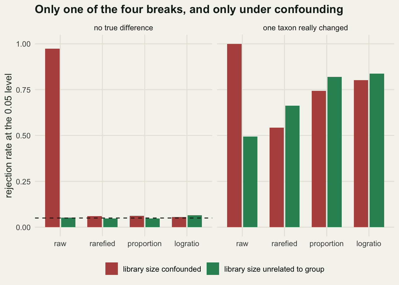

Figure 1: Type one error rate under a true null and power under a true 1.7 fold change, for four treatments of library size, in a regime where library size is unrelated to group and one where it is confounded with group. The dashed line is the nominal 0.05 rate.

The summary is the one McMurdie and Holmes reached for microbiome counts, in diet form. Rarefying is not invalid: it protects the error rate, and it is the cheapest thing to reach for when the depths are wildly unequal. It is wasteful, and the waste is measurable in power. Raw counts with no offset are the only option here that produces a wrong answer rather than a weak one, and they produce it silently. Standardising richness is a different question, where subsampling to equal coverage is the right move and rarefying to equal coverage is the tutorial for it. A differential abundance test does not need equal depth; it needs the depth out of the comparison, which is not the same operation.

Check two: one prey item drags the rest with it

The compositional trap has a specific form in a diet study. A prey item blooms, the predator eats a great deal of it in the second season, and every other prey item’s share of the reads falls because shares sum to one. Nothing else about the diet changed, and the test does not know that.

set.seed(414)
n_gb <- 25
gb <- rep(1:2, each = n_gb)
bloomer <- 4
fold <- 6
rise <- 2.4
cat("samples per group", n_gb, " blooming taxon", bloomer,
    " its baseline share", base_p[bloomer], " its true fold change", fold, "\n")

samples per group 25  blooming taxon 4  its baseline share 0.1  its true fold change 6 

sim_tab <- function(mult) {
  bio <- matrix(0, 2 * n_gb, n_taxa)
  for (k in seq_len(n_taxa)) bio[, k] <- base_p[k] * rlnorm(2 * n_gb, 0, 0.35)
  bio[gb == 2L, ] <- sweep(bio[gb == 2L, ], 2, mult, "*")
  lib <- round(rlnorm(2 * n_gb, log(40000), 0.35))
  pp <- bio / rowSums(bio)
  cnt <- matrix(0L, 2 * n_gb, n_taxa)
  for (i in seq_len(2 * n_gb)) cnt[i, ] <- as.integer(rmultinom(1, lib[i], pp[i, ]))
  list(cnt = cnt, tot = rowSums(cnt), bio = bio)
}

test_all <- function(s) {
  lg <- log(s$cnt + 0.5)
  scales_l <- list(proportion = log((s$cnt + 0.5) / (s$tot + 0.5 * n_taxa)),
                   logratio = lg - rowMeans(lg),
                   reference = lg - lg[, 1])
  lapply(scales_l, function(mm)
    t(sapply(seq_len(n_taxa), function(k) welch_p(mm[, k], gb))))
}

m_bloom <- rep(1, n_taxa); m_bloom[bloomer] <- fold
s_bloom <- sim_tab(m_bloom)
r_bloom <- test_all(s_bloom)
others <- setdiff(seq_len(n_taxa), bloomer)
cat("unchanged taxa in the table:", length(others), "\n")

unchanged taxa in the table: 11 

cat("of those, called significantly decreased:\n")

of those, called significantly decreased:

print(sapply(r_bloom, function(rr) sum(rr[others, "p"] < 0.05 & rr[others, "est"] < 0)))

proportion   logratio  reference 
        11          5          1 

cat("median estimated log change in the unchanged taxa:\n")

median estimated log change in the unchanged taxa:

print(round(sapply(r_bloom, function(rr) median(rr[others, "est"])), 3))

proportion   logratio  reference 
    -0.477     -0.199     -0.236 

cat("closure shift predicted for a proportion:",
    round(-log(1 + (fold - 1) * base_p[bloomer]), 3), "\n")

closure shift predicted for a proportion: -0.405 

cat("closure shift predicted for a centred log-ratio:",
    round(-log(fold) / n_taxa, 3),
    " and in a table of 60 taxa", round(-log(fold) / 60, 3), "\n")

closure shift predicted for a centred log-ratio: -0.149  and in a table of 60 taxa -0.03 

The log-ratio comes in two flavours here, so the comparison is three-way. The centred log-ratio divides each sample by its own geometric mean, which is the usual default. The reference log-ratio divides by one taxon, and the one used here is the most abundant prey item, which the simulation knows is unchanged.

The proportion test calls all 11 unchanged prey items significantly decreased. The centred log-ratio calls 5 of them. The reference log-ratio calls 1. The arithmetic behind those three numbers says how much protection a log-ratio buys. A sixfold rise in a prey item that held 0.1 of the diet inflates the total, so every other proportion falls by a factor whose log is -0.405, against a measured median shift of -0.477. The centred log-ratio subtracts the mean of the logs, and only one of the twelve logs moved, so the leak is the log of the fold change divided by the number of taxa: -0.149, against a measured median of -0.199. Smaller, but not zero, and with 25 samples per group it is large enough to be picked up in several of the unchanged taxa.

cat("everything rises by", rise, "fold, taxa called changed out of", n_taxa, "\n")

everything rises by 2.4 fold, taxa called changed out of 12 

s_all <- sim_tab(rep(rise, n_taxa))
r_all <- test_all(s_all)
print(sapply(r_all, function(rr) sum(rr[, "p"] < 0.05)))

proportion   logratio  reference 
         0          0          0 

cat("true total biomass ratio between groups",
    round(mean(rowSums(s_all$bio)[gb == 2L]) / mean(rowSums(s_all$bio)[gb == 1L]), 2),
    " read total ratio", round(mean(s_all$tot[gb == 2L]) / mean(s_all$tot[gb == 1L]), 2), "\n")

true total biomass ratio between groups 2.21  read total ratio 1.05 

n_rep_b <- 300
cnt_b <- matrix(0, n_rep_b, 6)
for (b in seq_len(n_rep_b)) {
  ra <- test_all(sim_tab(m_bloom))
  rb <- test_all(sim_tab(rep(rise, n_taxa)))
  cnt_b[b, 1:3] <- sapply(ra, function(rr)
    sum(rr[others, "p"] < 0.05 & rr[others, "est"] < 0))
  cnt_b[b, 4:6] <- sapply(rb, function(rr) sum(rr[, "p"] < 0.05))
}
cat("datasets simulated:", n_rep_b, "\n")

datasets simulated: 300 

cat("mean unchanged taxa called down under the bloom, out of", length(others), "\n")

mean unchanged taxa called down under the bloom, out of 11 

print(round(colMeans(cnt_b[, 1:3]), 2))

[1] 10.50  3.49  0.23

cat("mean taxa called changed when every taxon rose, out of", n_taxa, "\n")

mean taxa called changed when every taxon rose, out of 12 

print(round(colMeans(cnt_b[, 4:6]), 2))

[1] 0.47 0.53 0.46

Over 300 datasets the pattern holds: proportions call a mean of 10.5 of the 11 unchanged prey items decreased, the centred log-ratio 3.49, the reference log-ratio 0.23, which is the rate a correct test should give. That last number is the fix, and it comes with a condition the data cannot check: the reference has to be a taxon that did not change, and a read table says nothing about which taxon that is. Choosing one is an assumption, not an estimate.

The other direction is the one that gets left out. The second group eats 2.4 times as much of everything: total consumption rises, the proportions are identical, and the animals are in a genuinely different state. All three methods call 0 of the 12 taxa changed. The true total biomass ratio between groups is 2.21 and the ratio of read totals is 1.05, which is the sequencer answering a question about the flow cell rather than about the diet. No compositional method can detect this, because the information went when the libraries were pooled. It is the absence of a denominator, and the only repair comes from outside the read table: gut fullness, meal mass, a spike-in of known quantity.

prey_lab <- factor(paste("prey", seq_len(n_taxa)), levels = paste("prey", rev(seq_len(n_taxa))))
fig_b <- do.call(rbind, lapply(names(r_bloom), function(nm) {
  rr <- r_bloom[[nm]]
  data.frame(taxon = prey_lab, scale_used = nm,
             est = rr[, "est"], lo = rr[, "est"] - 1.96 * rr[, "se"],
             hi = rr[, "est"] + 1.96 * rr[, "se"])
}))
fig_b$scale_used <- factor(fig_b$scale_used, levels = c("proportion", "logratio", "reference"))
truth_b <- data.frame(taxon = factor(paste("prey", bloomer), levels = levels(prey_lab)),
                      est = log(fold))
ggplot(fig_b, aes(est, taxon, colour = scale_used)) +
  geom_vline(xintercept = 0, linetype = "dashed", colour = te_pal$ink) +
  geom_errorbarh(aes(xmin = lo, xmax = hi), height = 0,
                 position = position_dodge(width = 0.7)) +
  geom_point(size = 2, position = position_dodge(width = 0.7)) +
  geom_point(data = truth_b, aes(est, taxon), inherit.aes = FALSE,
             shape = 18, size = 4, colour = te_pal$gold) +
  scale_y_discrete(limits = levels(prey_lab)) +
  scale_colour_manual(values = c(proportion = te_pal$clay,
                                 logratio = te_pal$green,
                                 reference = te_pal$forest), name = NULL) +
  labs(title = "One prey item rose, eleven were called down",
       x = "estimated log change between groups", y = NULL) +
  theme_te() + theme(legend.position = "bottom")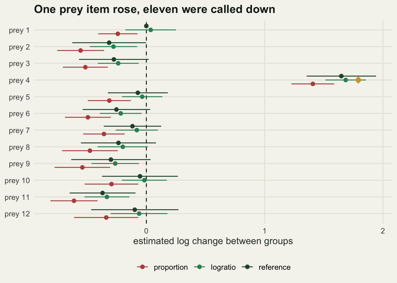

Warning: `geom_errorbarh()` was deprecated in ggplot2 4.0.0.
ℹ Please use the `orientation` argument of `geom_errorbar()` instead.

`height` was translated to `width`.

Figure 2: Estimated change in each prey item between groups when only prey 4 truly changed, on three scales, with 95 percent intervals. Truth is zero for every taxon except prey 4, whose true log change of 1.79 is the gold diamond. Prey 1 is the reference taxon, so its reference log-ratio is zero by construction.

Check three: replicates that are not replicates

A careful protocol takes several extractions from each faecal sample and several PCR replicates from each extraction, so the table has many more rows than the study has animals. Treating every row as an observation is tempting because it makes the sample size look excellent. Each level has its own variance: animals differ in what they ate, extractions in what they captured from a heterogeneous pellet, and PCR replicates in the stochastic amplification of low-copy templates.

set.seed(909)
n_animal <- 24
n_ext <- 3
n_pcr <- 3
sd_animal <- 0.45
sd_ext <- 0.30
sd_pcr <- 0.25
sd_small <- 0.12
n_rep_c <- 2000
gan <- rep(1:2, each = n_animal / 2)
gobs <- rep(gan, each = n_ext * n_pcr)
cat("animals", n_animal, " extractions each", n_ext, " PCRs each", n_pcr,
    " rows in the table", n_animal * n_ext * n_pcr, "\n")

animals 24  extractions each 3  PCRs each 3  rows in the table 216 

cat("sd animal", sd_animal, " sd extraction", sd_ext, " sd PCR", sd_pcr,
    " datasets per scenario", n_rep_c, "\n")

sd animal 0.45  sd extraction 0.3  sd PCR 0.25  datasets per scenario 2000 

icc_of <- function(sa) sa^2 / (sa^2 + sd_ext^2 + sd_pcr^2)
neff_of <- function(sa) n_animal * n_ext * n_pcr /
  (1 + (n_ext * n_pcr - 1) * icc_of(sa))
cat("intraclass correlation", round(icc_of(sd_animal), 3),
    " design effect", round(1 + (n_ext * n_pcr - 1) * icc_of(sd_animal), 2),
    " effective sample size", round(neff_of(sd_animal), 1), "\n")

intraclass correlation 0.57  design effect 5.56  effective sample size 38.8 

sim_hier <- function(sa, delta) {
  a <- rnorm(n_animal, 0, sa) + ifelse(gan == 2L, delta, 0)
  ee <- rnorm(n_animal * n_ext, 0, sd_ext)
  pp <- rnorm(n_animal * n_ext * n_pcr, 0, sd_pcr)
  a[rep(seq_len(n_animal), each = n_ext * n_pcr)] +
    ee[rep(seq_len(n_animal * n_ext), each = n_pcr)] + pp
}

run_hier <- function(sa, delta) {
  out <- matrix(0, n_rep_c, 4)
  for (b in seq_len(n_rep_c)) {
    y <- sim_hier(sa, delta)
    wn <- welch_p(y, gobs)
    am <- as.numeric(tapply(y, rep(seq_len(n_animal), each = n_ext * n_pcr), mean))
    wa <- welch_p(am, gan)
    out[b, ] <- c(wn[["p"]], wa[["p"]], wn[["est"]], wa[["est"]])
  }
  c(naive = mean(out[, 1] < 0.05), aggregated = mean(out[, 2] < 0.05),
    largest_estimate_gap = max(abs(out[, 3] - out[, 4])))
}

cat("null, animal sd", sd_animal, "\n")

null, animal sd 0.45 

print(round(run_hier(sd_animal, 0), 4))

               naive           aggregated largest_estimate_gap 
              0.4445               0.0495               0.0000 

cat("null, animal sd", sd_small, " intraclass correlation", round(icc_of(sd_small), 3),
    " effective sample size", round(neff_of(sd_small), 1), "\n")

null, animal sd 0.12  intraclass correlation 0.086  effective sample size 127.8 

print(round(run_hier(sd_small, 0), 4))

               naive           aggregated largest_estimate_gap 
              0.2325               0.0415               0.0000 

cat("power, animal sd", sd_small, " true group difference 0.25\n")

power, animal sd 0.12  true group difference 0.25

print(round(run_hier(sd_small, 0.25), 4))

               naive           aggregated largest_estimate_gap 
              0.9315               0.7220               0.0000 

Pooling all 216 rows as though they were independent rejects a true null 0.4445 of the time. The same data aggregated to 24 animal means rejects 0.0495 of the time, which is what a test at the 0.05 level should do. The intraclass correlation gives the size of the failure: with an animal standard deviation of 0.45 against 0.30 and 0.25 at the lower levels, 0.57 of the variance sits between animals, the design effect is 5.56, and 216 rows carry the information of 38.8 independent observations.

Weakening the animal term does not rescue the naive test. With an animal standard deviation of 0.12 the intraclass correlation drops to 0.086 and the effective sample size rises to 127.8, and the naive test still rejects a true null 0.2325 of the time. The aggregated test holds at 0.0415.

What aggregation costs shows up in the same scenario. With a true group difference of 0.25 and a small animal variance, the naive test has power 0.9315 and the aggregated test 0.722. That gap is real but it is not a bargain: the extra power is bought at an error rate of 0.2325. The two tests agree exactly on the estimate, and the largest gap between their point estimates over 2000 datasets is 0. With a balanced design that is no coincidence: they are the same difference of means, and only the standard error differs.

budget_rx <- n_animal * n_ext * n_pcr
alloc <- expand.grid(ext = 1:3, pcr = 1:3)
alloc$animals <- floor(budget_rx / (alloc$ext * alloc$pcr))
for (nm in c("large", "small")) {
  sa <- if (nm == "large") sd_animal else sd_small
  vv <- sa^2 + sd_ext^2 / alloc$ext + sd_pcr^2 / (alloc$ext * alloc$pcr)
  alloc[[nm]] <- sqrt(2 * vv / (alloc$animals / 2))
}
cat("fixed budget of PCR reactions:", budget_rx, "\n")

fixed budget of PCR reactions: 216 

print(alloc[order(alloc$large), ], row.names = FALSE, digits = 3)

 ext pcr animals  large  small
   1   1     216 0.0811 0.0556
   2   1     108 0.1016 0.0579
   1   2     108 0.1095 0.0709
   3   1      72 0.1186 0.0602
   1   3      72 0.1319 0.0834
   2   2      54 0.1396 0.0745
   3   2      36 0.1643 0.0780
   2   3      36 0.1693 0.0881
   3   3      24 0.1998 0.0925

cat("worst over best allocation, large animal variance:",
    round(max(alloc$large) / min(alloc$large), 2),
    " small animal variance:", round(max(alloc$small) / min(alloc$small), 2), "\n")

worst over best allocation, large animal variance: 2.46  small animal variance: 1.66 

The design question is which level of replication buys precision, and the variance of an animal mean answers it: the animal term is divided by nothing, the extraction term by the number of extractions, and the PCR term by their product. Holding the number of PCR reactions fixed at 216, one extraction and one PCR from each of 216 animals gives a standard error of 0.0811 on the group difference, while three extractions and three PCRs from each of 24 animals gives 0.1998, worse by a factor of 2.46. With a small animal variance the ordering holds and the gap narrows to 1.66. Sub-sampling within an animal cannot touch the between-animal term, and that term is most of the variance in every scenario tried here.

scen_lv <- c("animal sd 0.45", "animal sd 0.12")
fig_c <- rbind(
  data.frame(animals = alloc$animals, se_val = alloc$large,
             lab = paste(alloc$ext, "x", alloc$pcr), scenario = scen_lv[1]),
  data.frame(animals = alloc$animals, se_val = alloc$small,
             lab = paste(alloc$ext, "x", alloc$pcr), scenario = scen_lv[2]))
fig_c$scenario <- factor(fig_c$scenario, levels = scen_lv)
ggplot(fig_c, aes(animals, se_val)) +
  geom_point(size = 2.6, colour = te_pal$forest) +
  geom_text(aes(label = lab), size = 3, vjust = -0.9, colour = te_pal$ink) +
  facet_wrap(~scenario) +
  scale_x_log10(expand = expansion(mult = 0.16)) +
  scale_y_continuous(expand = expansion(mult = c(0.08, 0.16))) +
  labs(title = "Animals buy precision; replicates of an animal buy less",
       x = "animals in the study (log scale)",
       y = "standard error of the group difference") +
  theme_te()

Figure 3: Standard error of the estimated group difference against the number of animals, for nine ways of spending a fixed budget of 216 PCR reactions, under a large and a small animal variance. Labels give extractions per animal and PCR replicates per extraction.

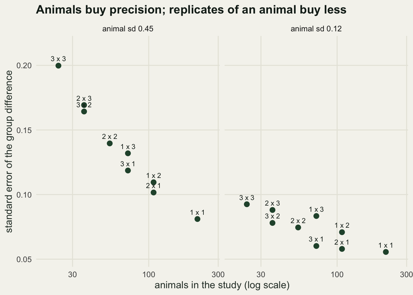
The honest limit on that table is that it treats a PCR replicate as a noisy measurement of a continuous log-ratio. Replicates also decide whether a rare prey item is detected at all, which this variance calculation cannot see: a taxon in one replicate out of three is a different kind of observation from one in all three, and Ficetola and colleagues built the replication design for that presence and absence problem. If the study reports occurrence, replicates are buying detection probability rather than precision, and the arithmetic above does not apply.

Check four: the depth at which a diet is complete

The last check is the one a reviewer asks about most often and a paper answers least often: was the sequencing deep enough. A population of 2000 animals is simulated with a pool of 30 prey taxa, uneven within each animal the way real diets are, so the smallest prey share in a typical animal is under one part in ten thousand. Sixty animals are sequenced to 100000 reads, then rarefied down a grid of depths.

set.seed(7311)
n_prey <- 30
n_pop <- 2000
prey_prev <- seq(0.85, 0.10, length.out = n_prey)
pres <- matrix(runif(n_pop * n_prey) < rep(prey_prev, each = n_pop), n_pop, n_prey)
pres[cbind(seq_len(n_pop), max.col(matrix(runif(n_pop * n_prey), n_pop, n_prey)))] <- TRUE
wt <- matrix(rlnorm(n_pop * n_prey, 0, 2.6), n_pop, n_prey) * pres
pop_w <- wt / rowSums(wt)
rich_true <- rowSums(pop_w > 0)
even_true <- apply(pop_w, 1, function(w) {
  w <- w[w > 0]; -sum(w * log(w)) / log(length(w))
})
cat("animals in the population", n_pop, " prey pool", n_prey, "\n")

animals in the population 2000  prey pool 30 

cat("prey per animal, median", median(rich_true),
    " range", min(rich_true), "to", max(rich_true), "\n")

prey per animal, median 15  range 5 to 24 

cat("evenness median", round(median(even_true), 3),
    " smallest prey share in the median animal",
    signif(median(apply(pop_w, 1, function(w) min(w[w > 0]))), 2), "\n")

evenness median 0.496  smallest prey share in the median animal 8.1e-05 

n_sub <- 60
idx_sub <- sample(n_pop, n_sub)
deep <- 100000
dep_grid <- c(200, 500, 1000, 2000, 5000, 10000, 20000, 50000, 100000)
deep_lib <- matrix(0L, n_sub, n_prey)
for (i in seq_len(n_sub)) {
  deep_lib[i, ] <- as.integer(rmultinom(1, deep, pop_w[idx_sub[i], ]))
}
det_frac <- matrix(0, n_sub, length(dep_grid))
for (i in seq_len(n_sub)) for (j in seq_along(dep_grid)) {
  det_frac[i, j] <- sum(rarefy_row(deep_lib[i, ], dep_grid[j]) > 0) / rich_true[idx_sub[i]]
}
cat("samples sequenced", n_sub, " deepest library", deep, "\n")

samples sequenced 60  deepest library 1e+05 

cat("median fraction of a sample's prey detected, by depth:\n")

median fraction of a sample's prey detected, by depth:

print(round(apply(det_frac, 2, median), 3))

[1] 0.613 0.733 0.833 0.875 0.933 1.000 1.000 1.000 1.000

d95_of <- function(fr) {
  ok <- which(fr >= 0.95)
  if (!length(ok)) return(NA_real_)
  j <- ok[1]
  if (j == 1) return(dep_grid[1])
  x1 <- log(dep_grid[j - 1]); x2 <- log(dep_grid[j])
  exp(x1 + (0.95 - fr[j - 1]) * (x2 - x1) / (fr[j] - fr[j - 1]))
}
d95 <- apply(det_frac, 1, d95_of)
cat("median depth reaching 95 percent of a sample's prey:",
    round(median(d95, na.rm = TRUE)), "\n")

median depth reaching 95 percent of a sample's prey: 3466 

cat("samples that never reach it, even at", deep, "reads:", sum(is.na(d95)), "\n")

samples that never reach it, even at 1e+05 reads: 9 

ev_sub <- even_true[idx_sub]
lo_half <- ev_sub <= median(ev_sub)
cat("uneven half: evenness", round(median(ev_sub[lo_half]), 3),
    " dominant prey share", round(median(apply(pop_w[idx_sub[lo_half], ], 1, max)), 3),
    " depth", round(median(d95[lo_half], na.rm = TRUE)), "\n")

uneven half: evenness 0.395  dominant prey share 0.669  depth 7711 

cat("even half: evenness", round(median(ev_sub[!lo_half]), 3),
    " dominant prey share", round(median(apply(pop_w[idx_sub[!lo_half], ], 1, max)), 3),
    " depth", round(median(d95[!lo_half], na.rm = TRUE)), "\n")

even half: evenness 0.596  dominant prey share 0.385  depth 3426 

The median sample needs 6373 reads to recover 95 percent of the prey items it actually contains, and 10 of the 60 never get there within 100000 reads, because they hold a prey item too rare to be sampled reliably at any depth a run can afford. The median alone is not the useful number, though. Split the samples at the median evenness and the requirement splits with them: the uneven half, whose dominant prey holds 0.669 of the diet, needs 9148 reads, and the even half, whose dominant prey holds 0.385, needs 3554. Those are medians of the per-sample requirement rather than the crossing point of the median curve, which sits higher. A gut full of one fish hides its minor prey behind that fish, and the only way past it is more reads. Alberdi and colleagues reach the same conclusion from real runs rather than simulated ones, with replicate number and sequencing depth examined together.

fig_d <- data.frame(depth = rep(dep_grid, each = n_sub),
                    frac = as.vector(det_frac),
                    id = rep(seq_len(n_sub), times = length(dep_grid)),
                    half = rep(ifelse(lo_half, "less even half", "more even half"),
                               times = length(dep_grid)))
med_d <- aggregate(frac ~ depth + half, data = fig_d, FUN = median)
ggplot(fig_d, aes(depth, frac)) +
  geom_line(aes(group = id), colour = te_pal$line, linewidth = 0.4) +
  geom_hline(yintercept = 0.95, linetype = "dashed", colour = te_pal$ink) +
  geom_line(data = med_d, aes(colour = half), linewidth = 1.1) +
  geom_point(data = med_d, aes(colour = half), size = 2) +
  scale_colour_manual(values = c("less even half" = te_pal$clay,
                                 "more even half" = te_pal$green), name = NULL) +
  scale_x_log10() +
  labs(title = "Evenness sets the depth a sample needs",
       x = "reads per sample (log scale)",
       y = "fraction of the sample's prey detected") +
  theme_te() + theme(legend.position = "bottom")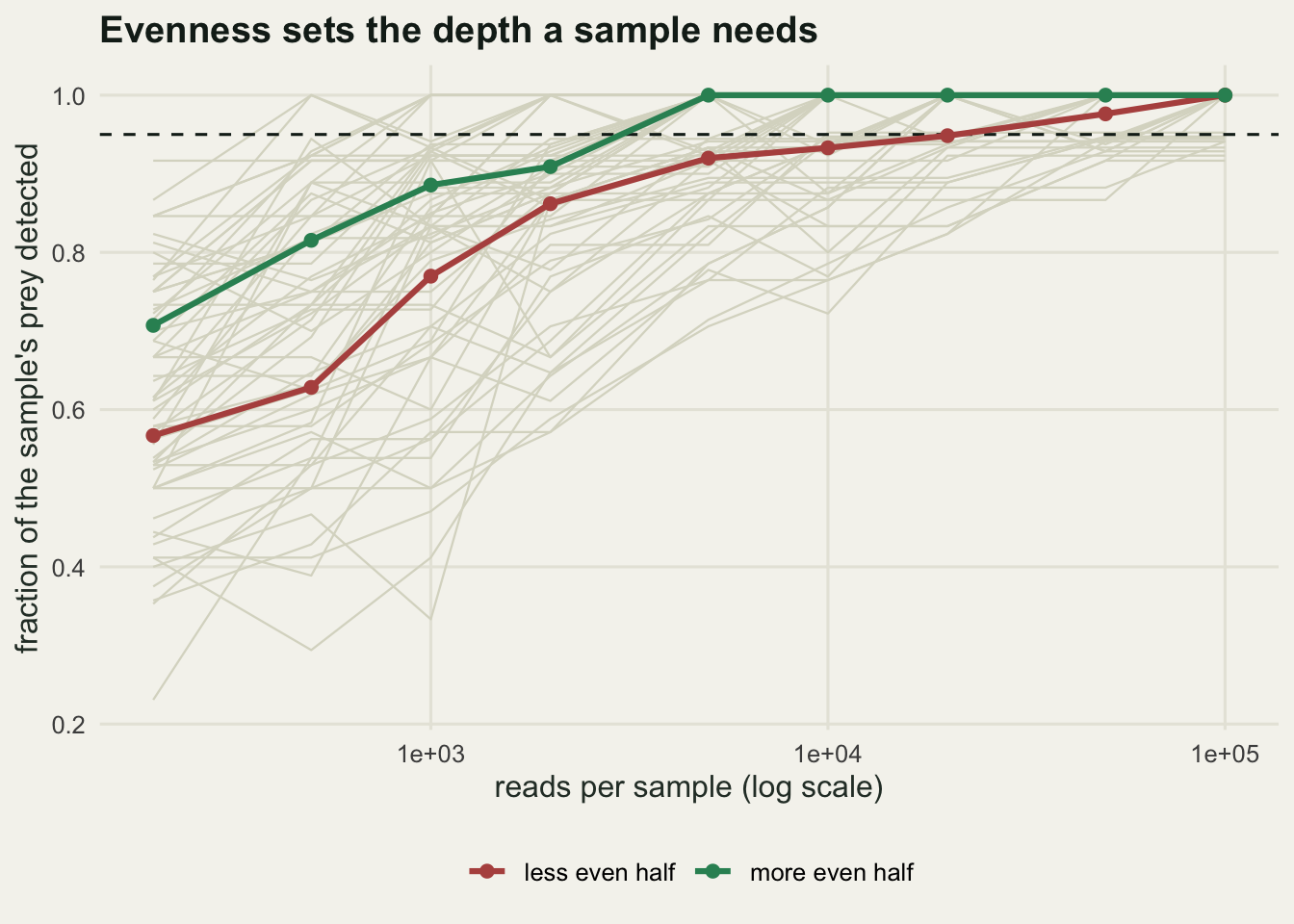

Figure 4: Fraction of a sample’s true prey items detected against sequencing depth. Grey lines are the 60 samples; the coloured lines are the median detection curves of the less even and the more even half. The dashed line marks 95 percent completeness.

That per-sample number is not the design question. A run has a fixed capacity, and spending it on depth means spending fewer animals. The comparison below fixes the total at 3.2 million reads and splits it every way from 40 animals at 80000 reads to 1280 animals at 2500 reads, scoring each allocation on a population-level summary rather than a per-sample one: the mean absolute error of the estimated frequency of occurrence across the 30 prey taxa, and the same error for the mean dietary composition.

budget_reads <- 3.2e6
n_grid <- c(40, 80, 160, 320, 640, 1280)
n_studies <- 40
foo_true <- colMeans(pop_w > 0)
comp_true <- colMeans(pop_w)
res_d <- data.frame(samples = n_grid, depth = round(budget_reads / n_grid),
                    occurrence = 0, composition = 0)
for (s in seq_along(n_grid)) {
  ns <- n_grid[s]; dp <- round(budget_reads / ns)
  fm <- numeric(n_studies); cm <- numeric(n_studies)
  for (b in seq_len(n_studies)) {
    ii <- sample(n_pop, ns)
    tabs <- matrix(0L, ns, n_prey)
    for (i in seq_len(ns)) tabs[i, ] <- as.integer(rmultinom(1, dp, pop_w[ii[i], ]))
    fm[b] <- mean(abs(colMeans(tabs > 0) - foo_true))
    cm[b] <- mean(abs(colMeans(tabs / rowSums(tabs)) - comp_true))
  }
  res_d$occurrence[s] <- mean(fm)
  res_d$composition[s] <- mean(cm)
}
cat("total reads", budget_reads, " simulated studies per allocation", n_studies, "\n")

total reads 3200000  simulated studies per allocation 40 

print(res_d, row.names = FALSE, digits = 3)

 samples depth occurrence composition
      40 80000     0.0572     0.01443
      80 40000     0.0420     0.00980
     160 20000     0.0318     0.00684
     320 10000     0.0345     0.00453
     640  5000     0.0489     0.00277
    1280  2500     0.0703     0.00151

cat("best occurrence allocation:", res_d$samples[which.min(res_d$occurrence)],
    "samples at", res_d$depth[which.min(res_d$occurrence)], "reads\n")

best occurrence allocation: 160 samples at 20000 reads

cat("occurrence error, deepest over best:",
    round(res_d$occurrence[1] / min(res_d$occurrence), 2),
    " shallowest over best:",
    round(res_d$occurrence[length(n_grid)] / min(res_d$occurrence), 2), "\n")

occurrence error, deepest over best: 1.8  shallowest over best: 2.21 

cat("composition error, deepest over shallowest:",
    round(res_d$composition[1] / res_d$composition[length(n_grid)], 2), "\n")

composition error, deepest over shallowest: 9.58 

For the composition summary the answer is one-directional and not close: the error falls from 0.01417 at 40 deep samples to 0.00152 at 1280 shallow ones, a factor of 9.35, and every step towards more animals improves it. A mean proportion is unbiased at any depth, so the only limit is how many animals the study looked at.

For occurrence the answer has an interior optimum, at 160 samples of 20000 reads with an error of 0.0326. Going deeper costs: the 40-sample corner is 1.74 times worse. Going shallower costs more, because at 2500 reads a prey item at one part in ten thousand is usually missed and occurrence is biased downwards for every taxon at once, giving 2.16 times the error of the optimum. That optimum depth sits above the 6373 reads the median sample needed for its own completeness, which is what you would expect from a summary that needs the rare prey seen in every animal that ate it.

Most diet protocols sequence a modest number of samples as deeply as the run allows, and on this simulation that is the losing corner. Shallow-and-many wins outright for composition and beats deep-and-few for occurrence as well. The design that loses is the one with 40 animals in it.

What none of these checks can catch

Every check above tests an analysis against the read table it was given. That is the whole of what they can do, and the read table is not the diet.

None of them can tell whether the marker amplifies the prey that matter. A primer pair that misses a whole class of prey produces a table with no anomaly in it: the missing taxa are simply not there, the remaining ratios are internally consistent, and every diagnostic above passes. None of them can tell whether the reference database contains the species that were eaten, because an unmatched sequence is silently absent rather than flagged, so a well-sequenced prey item with no reference entry disappears exactly like a prey item that was never eaten. None of them can separate secondary predation from primary: the stomach contents of a fish the predator ate arrive in the same pellet, amplify with the same primers, and appear as prey of the predator. And none can see what digestion destroyed before extraction, which is systematically the soft-bodied and the small.

A diet study can pass all four of these checks and describe a diet that is wrong in the direction of whatever the marker sees best. The checks measure whether the statistics are honest about the table. They say nothing about whether the table is honest about the animal. The instruments for that are different: mock communities of known composition run through the same pipeline, a second marker, a reference database whose coverage of the local fauna has been counted rather than assumed, and a comparison against a method that does not use DNA at all.

Where to go next

This closes the metabarcoding cluster. The first post left a read table whose row totals carry no dietary information, and check one says what to do with those totals in a test. The second left amplification bias as a per taxon multiplier, and check two says that one blooming prey item does damage of the same kind through closure alone, with no bias needed. The third left a filtered table, and checks three and four say what the replicate structure and the depth behind it were worth.

Sideways from here, the same molecular detection problem framed as occupancy is in eDNA occupancy with three levels, where the hierarchy of check three becomes the model rather than a nuisance, and a replicate that fails to detect is data rather than a zero to be filtered.

References

McMurdie PJ, Holmes S 2014 PLoS Computational Biology 10(4):e1003531 (10.1371/journal.pcbi.1003531)

Weiss S, Xu ZZ, Peddada S, Amir A, Bittinger K, Gonzalez A, Lozupone C, Zaneveld JR, Vazquez-Baeza Y, Birmingham A, Hyde ER, Knight R 2017 Microbiome 5:27 (10.1186/s40168-017-0237-y)

Gloor GB, Macklaim JM, Pawlowsky-Glahn V, Egozcue JJ 2017 Frontiers in Microbiology 8:2224 (10.3389/fmicb.2017.02224)

Deagle BE, Thomas AC, McInnes JC, Clarke LJ, Vesterinen EJ, Clare EL, Kartzinel TR, Eveson JP 2019 Molecular Ecology 28(2):391-406 (10.1111/mec.14734)

Alberdi A, Aizpurua O, Gilbert MTP, Bohmann K 2018 Methods in Ecology and Evolution 9(1):134-147 (10.1111/2041-210X.12849)

Ficetola GF, Pansu J, Bonin A, Coissac E, Giguet-Covex C, De Barba M, Gielly L, Lopes CM, Boyer F, Pompanon F, Raye G, Taberlet P 2015 Molecular Ecology Resources 15(3):543-556 (10.1111/1755-0998.12338)

Related tutorials

• Metabarcoding reads as compositional data
• PCR bias and amplification efficiency
• Contamination filtering in metabarcoding
• Checking a compositional analysis