Metabarcoding reads as compositional data

A simulated diet study in R showing why DNA metabarcoding read counts are compositional, and how relative read abundance and occurrence summaries fail.

A metabarcoding run hands you a matrix: samples down the rows, prey taxa across the columns, read counts in the cells. The counts look like abundances and get treated like abundances. They are not. The total in each row was fixed when the run was loaded: the flow cell has a capacity, that capacity is divided among the samples in the pool, and whatever quantity of prey DNA came out of a given gut was normalised away when the libraries were pooled to equal molarity. An animal that ate twenty grams and one that ate two hundred come back with read totals of the same size.

What survives is the set of ratios inside a row, and a table whose rows carry only ratios is a composition. The generic consequences of that are covered elsewhere on this blog: closure, the correlations it manufactures, and the log-ratio transformations that undo them are in Log-ratio transformations: clr, alr and ilr, which is the prerequisite for this one. Here the subject is narrower: the two summaries that every diet paper reports, relative read abundance (RRA) and frequency of occurrence (FOO), answer different questions, and they fail in ways that have nothing in common.

To see how they fail you need a diet whose truth you already know. The simulation below builds one: a set of faecal or gut samples with a known biomass composition, pushed through the steps that sit between a mouthful and a read count. It then measures the row total against what the animal ate, RRA against the truth within and between taxa, FOO against true occurrence, the score of RRA, percentage of occurrence (POO) and weighted POO on two criteria, and how far the detection threshold moves the answer.

From bite to read count

The true diet is ten prey taxa across one hundred and twenty animals. Each taxon has a prevalence (the fraction of animals that ate it at all) and a median meal size in grams, loosely related as they are in a real diet, with two deliberate exceptions: amphipods are in every gut in trace amounts, and herring is in fewer guts but in bulk. A per animal fullness multiplier scales the whole meal up or down, so the quantity eaten varies far more than the composition does.

library(ggplot2)

te_pal <- list(forest = "#275139", green = "#2f8f63", sage = "#93a87f",
               clay = "#b5534e", gold = "#cda23f", line = "#dad9ca",
               ink = "#16241d", paper = "#f5f4ee")

theme_te <- function() {
  theme_minimal(base_size = 12) +
    theme(panel.grid.minor = element_blank(),
          panel.grid.major = element_line(colour = "#e7e6dc"),
          plot.background = element_rect(fill = "#f5f4ee", colour = NA),
          panel.background = element_rect(fill = "#f5f4ee", colour = NA),
          plot.title = element_text(face = "bold", colour = te_pal$ink),
          axis.title = element_text(colour = "#2c3a31"))
}

set.seed(20260817)
taxon_lab <- c("krill", "sandeel", "herring", "polychaete", "shrimp",
               "mysid", "squid", "amphipod", "isopod", "copepod")
n_taxa <- length(taxon_lab)
n_samples <- 120
prev_true <- c(1.00, 0.92, 0.72, 0.62, 0.55, 0.48, 0.38, 1.00, 0.30, 0.26)
mass_med <- c(16, 8, 6, 4, 3, 2.2, 2.0, 0.28, 2.2, 1.0)
cat("taxa:", n_taxa, " samples:", n_samples, "\n")

taxa: 10  samples: 120 

cat("prevalence from", min(prev_true), "to", max(prev_true), "\n")

prevalence from 0.26 to 1 

cat("median meal size (g) from", min(mass_med), "to", max(mass_med), "\n")

median meal size (g) from 0.28 to 16 

biomass <- matrix(0, n_samples, n_taxa, dimnames = list(NULL, taxon_lab))
fullness <- rlnorm(n_samples, 0, 0.85)
for (k in seq_len(n_taxa)) {
  biomass[, k] <- rbinom(n_samples, 1, prev_true[k]) *
    rlnorm(n_samples, log(mass_med[k]), 0.55) * fullness
}
gut_total <- rowSums(biomass)
w_true <- biomass / gut_total
mean_w <- colMeans(w_true)
occ_true <- colMeans(biomass > 0)
cat("gut contents (g), smallest and largest:",
    round(min(gut_total), 1), round(max(gut_total), 1), "\n")

gut contents (g), smallest and largest: 4.5 664.2 

cat("ratio of largest to smallest:", round(max(gut_total) / min(gut_total), 1), "\n")

ratio of largest to smallest: 146.2 

Between that biomass and the read table sit three steps. The first is DNA yield: a gram of copepod and a gram of herring muscle do not release the same number of marker copies, because cell size, mitochondrial copy number and how far digestion has gone all differ by taxon. The second is amplification: primers sit better on some templates than on others, so a copy of one template is not worth a copy of another by the end of the PCR. Both are modelled here as one multiplicative factor per taxon, and their product is the recovery factor. That single number for amplification is a deliberate simplification; the next tutorial in this cluster takes the PCR apart properly.

yield_k <- rlnorm(n_taxa, 0, 0.55)
eff_k <- rlnorm(n_taxa, 0, 0.35)
yield_k <- yield_k / exp(mean(log(yield_k)))
eff_k <- eff_k / exp(mean(log(eff_k)))
recovery <- yield_k * eff_k
names(recovery) <- taxon_lab
print(round(recovery, 3))

     krill    sandeel    herring polychaete     shrimp      mysid      squid 
     0.750      1.030      4.543      0.549      1.338      1.338      0.752 
  amphipod     isopod    copepod 
     1.149      0.577      0.582 

cat("largest over smallest recovery factor:",
    round(max(recovery) / min(recovery), 2), "\n")

largest over smallest recovery factor: 8.28 

The third step is the sequencer. Each sample gets a read total drawn from the run, and the reads are allocated across taxa by a multinomial draw with probabilities proportional to the amplified DNA. The read total varies from library to library, but it varies for reasons of pooling and cluster density, not because of what the animal ate.

lib_size <- round(rlnorm(n_samples, log(46000), 0.20))
p_expect <- sweep(biomass, 2, recovery, "*")
p_expect <- p_expect / rowSums(p_expect)
reads <- matrix(0L, n_samples, n_taxa, dimnames = list(NULL, taxon_lab))
for (i in seq_len(n_samples)) {
  reads[i, ] <- as.integer(rmultinom(1, lib_size[i], p_expect[i, ]))
}
read_total <- rowSums(reads)
rra <- reads / read_total
mean_rra <- colMeans(rra)
cat("read totals, smallest and largest:", min(read_total), max(read_total), "\n")

read totals, smallest and largest: 26297 88082 

The recovery factors span a factor of 8.28 in this draw, from 0.549 for the soft-bodied polychaete to 4.543 for herring. That is not an extreme choice: published comparisons of read proportions against known tissue mixtures routinely find taxon effects of that size and larger.

The library size carries no dietary information

Take the animal fifteenth from the bottom in gut mass, and the animal whose gut mass is closest to ten times larger. The one ate 13.8 g and the other 138.6 g, a ratio of 10.05. Their read totals are 32785 and 60526, a ratio of 1.85 in the same direction, which looks like a signal until you notice that read totals in this run scatter across a similar range for animals of every size.

ord <- order(gut_total)
i_low <- ord[15]
i_high <- which.min(abs(gut_total - 10 * gut_total[i_low]))
cat("animal A ate", round(gut_total[i_low], 1), "g and returned",
    read_total[i_low], "reads\n")

animal A ate 13.8 g and returned 32785 reads

cat("animal B ate", round(gut_total[i_high], 1), "g and returned",
    read_total[i_high], "reads\n")

animal B ate 138.6 g and returned 60526 reads

cat("biomass ratio", round(gut_total[i_high] / gut_total[i_low], 2),
    " read ratio", round(read_total[i_high] / read_total[i_low], 2), "\n")

biomass ratio 10.05  read ratio 1.85 

cat("sd of log gut mass", round(sd(log(gut_total)), 3),
    " sd of log read total", round(sd(log(read_total)), 3), "\n")

sd of log gut mass 0.981  sd of log read total 0.212 

ct <- cor.test(log(gut_total), log(read_total))
cat("correlation", round(ct$estimate, 3), " p", round(ct$p.value, 3), "\n")

correlation -0.077  p 0.406 

The correlation between log gut mass and log read total is -0.077 with a p value of 0.406, and the spread of the two quantities is not comparable: the standard deviation of log gut mass is 0.981 against 0.212 for log read total. Gut contents in this simulation range over a factor of 146.2; read totals were drawn from a distribution that knows nothing about them. Searching for a pair of animals whose gut masses differ by at least eightfold and whose read totals are as close as possible finds one that makes the point without any statistics.

gap_ok <- outer(gut_total, gut_total, "/") >= 8
read_gap <- abs(outer(log(read_total), log(read_total), "-"))
read_gap[!gap_ok] <- Inf
hit <- which(read_gap == min(read_gap), arr.ind = TRUE)[1, ]
cat("animal C:", round(gut_total[hit[1]], 1), "g and", read_total[hit[1]], "reads\n")

animal C: 248.6 g and 51280 reads

cat("animal D:", round(gut_total[hit[2]], 1), "g and", read_total[hit[2]], "reads\n")

animal D: 22.8 g and 51284 reads

cat("biomass ratio:", round(gut_total[hit[1]] / gut_total[hit[2]], 2), "\n")

biomass ratio: 10.9 

lib_df <- data.frame(gut = gut_total, reads = read_total,
                     marked = seq_len(n_samples) %in% hit)
pair_df <- data.frame(gut = gut_total[hit], reads = read_total[hit])
ggplot(lib_df, aes(gut, reads)) +
  geom_line(data = pair_df, colour = te_pal$clay, linetype = "dashed") +
  geom_point(aes(colour = marked, size = marked), alpha = 0.85) +
  scale_colour_manual(values = c("FALSE" = te_pal$sage, "TRUE" = te_pal$clay),
                      guide = "none") +
  scale_size_manual(values = c("FALSE" = 1.9, "TRUE" = 3.4), guide = "none") +
  scale_x_log10() +
  labs(x = "gut contents consumed (g, log scale)",
       y = "reads returned for the sample", title = "The sequencer sets the row total") +
  theme_te()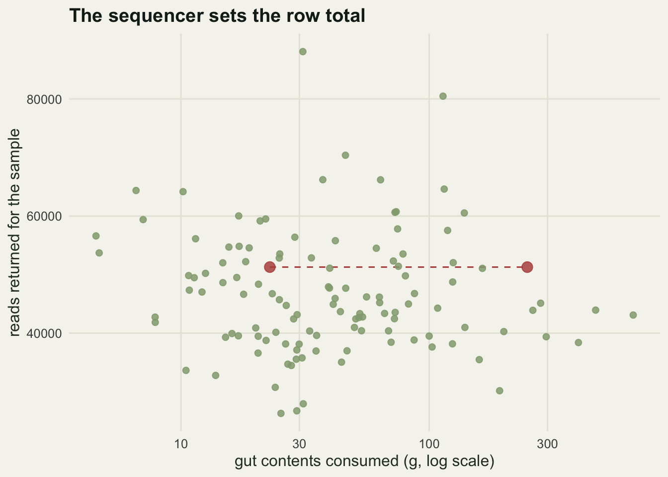

Figure 1: Reads returned per sample against the biomass the animal actually consumed. The two highlighted animals differ elevenfold in gut contents and by four reads in library size.

Animal C ate 248.6 g and returned 51280 reads. Animal D ate 22.8 g and returned 51284 reads. The consequence is the whole reason this post exists: a read count is interpretable only relative to the other reads in its own sample. Absolute counts cannot be compared across samples, and a count is not a quantity of prey. That is exactly what makes the table compositional.

Relative read abundance against the truth

Relative read abundance is the read count divided by the sample total. Regress it on the true biomass proportion across every taxon and every sample and the fit looks respectable: a slope of 0.840 and a correlation of 0.800. That respectability is the trap.

pooled <- lm(as.vector(rra) ~ as.vector(w_true))
cat("pooled slope", round(coef(pooled)[2], 3),
    " intercept", round(coef(pooled)[1], 3),
    " correlation", round(cor(as.vector(rra), as.vector(w_true)), 3), "\n")

pooled slope 0.84  intercept 0.016  correlation 0.8 

within_r <- vapply(seq_len(n_taxa), function(k) {
  ok <- w_true[, k] > 0
  cor(rra[ok, k], w_true[ok, k])
}, numeric(1))
names(within_r) <- taxon_lab
cat("within-taxon correlation, median", round(median(within_r), 3),
    " lowest", round(min(within_r), 3), "\n")

within-taxon correlation, median 0.911  lowest 0.857 

offset_k <- colSums(rra) / colSums(w_true)
print(round(offset_k, 3))

     krill    sandeel    herring polychaete     shrimp      mysid      squid 
     0.683      0.916      2.998      0.529      1.157      1.121      0.652 
  amphipod     isopod    copepod 
     1.026      0.495      0.543 

cat("largest offset:", names(which.max(offset_k)), round(max(offset_k), 2), "\n")

largest offset: herring 3 

cat("smallest offset:", names(which.min(offset_k)), round(min(offset_k), 2), "\n")

smallest offset: isopod 0.49 

cat("offset spread", round(max(offset_k) / min(offset_k), 2),
    " recovery spread", round(max(recovery) / min(recovery), 2), "\n")

offset spread 6.06  recovery spread 8.28 

cat("correlation of log offset with log recovery",
    round(cor(log(offset_k), log(recovery)), 3), "\n")

correlation of log offset with log recovery 0.997 

Within a taxon, RRA does track the truth: the median correlation between a taxon’s RRA and its true biomass share across animals is 0.910, and the lowest of the ten is 0.854. An animal that ate more herring relative to everything else does return proportionally more herring reads. The damage is between taxa. The multiplicative offset, defined here as the summed RRA over the summed true share, runs from 0.50 for isopod to 3.00 for herring. Two taxa with identical shares of the real diet come out of the pipeline a factor of 6.05 apart.

Those offsets are the recovery factors showing through: their logarithms correlate at 0.997. They are not equal to the recovery factors, though. The recovery factors span 8.28 and the offsets only 6.05, because closure drags every offset towards one. A taxon’s read share depends on its own recovery factor and on the recovery factors of whatever else was in the same gut, so even the bias is not a clean per taxon constant.

cat("krill: true share", round(mean_w["krill"], 4),
    " RRA", round(mean_rra["krill"], 4), "\n")

krill: true share 0.4428  RRA 0.3027 

cat("herring: true share", round(mean_w["herring"], 4),
    " RRA", round(mean_rra["herring"], 4), "\n")

herring: true share 0.1024  RRA 0.3071 

cat("true ratio krill to herring", round(mean_w["krill"] / mean_w["herring"], 2),
    " RRA ratio", round(mean_rra["krill"] / mean_rra["herring"], 3), "\n")

true ratio krill to herring 4.32  RRA ratio 0.986 

The practical cost is a bar chart that names the wrong top prey. Krill is 0.4428 of the diet by biomass and herring 0.1024, a ratio of 4.32. In RRA they are 0.3026 and 0.3071: herring edges ahead, and the two are within 2 percent of each other. A ranking of taxa by RRA is a ranking distorted by recovery, and the distortion is large enough to reorder the top of the list.

Frequency of occurrence and its ceiling

Frequency of occurrence asks a different question: in what fraction of samples does the taxon appear at all, above some read threshold. Set that threshold at 0.1 percent of the sample’s reads and FOO is not approximately right, it is exactly right for all ten taxa.

thr_base <- 0.001
detected <- rra >= thr_base
foo <- colMeans(detected)
cat("largest gap between FOO and true occurrence:",
    round(max(abs(foo - occ_true)), 4), "\n")

largest gap between FOO and true occurrence: 0 

smry <- data.frame(occurrence = round(occ_true, 3), foo = round(foo, 3),
                   true_share = round(mean_w, 4), rra = round(mean_rra, 4),
                   recovery = round(recovery, 2))
print(smry)

           occurrence   foo true_share    rra recovery
krill           1.000 1.000     0.4428 0.3027     0.75
sandeel         0.925 0.925     0.2304 0.2110     1.03
herring         0.650 0.650     0.1024 0.3071     4.54
polychaete      0.583 0.583     0.0701 0.0370     0.55
shrimp          0.558 0.558     0.0529 0.0613     1.34
mysid           0.517 0.517     0.0346 0.0387     1.34
squid           0.383 0.383     0.0249 0.0162     0.75
amphipod        1.000 1.000     0.0090 0.0092     1.15
isopod          0.300 0.300     0.0225 0.0111     0.58
copepod         0.300 0.300     0.0104 0.0056     0.58

That is the case for FOO in one line: the recovery factors span more than eightfold and every frequency comes back without error, because a taxon that is present clears a low threshold whatever its amplification efficiency. FOO is free of the recovery factors in practice rather than in principle, at a sensible threshold and away from the detection limit, which is a point the threshold sweep below will spoil.

The price is that FOO saturates. It counts guts, not grams, and a gut that contained a milligram of a taxon counts the same as a gut stuffed with it.

pair_idx <- t(combn(n_taxa, 2))
foo_gap <- abs(foo[pair_idx[, 1]] - foo[pair_idx[, 2]])
rra_ratio <- pmax(mean_rra[pair_idx[, 1]], mean_rra[pair_idx[, 2]]) /
  pmin(mean_rra[pair_idx[, 1]], mean_rra[pair_idx[, 2]])
tie_foo <- which(foo_gap < 0.01)
best_a <- tie_foo[which.max(rra_ratio[tie_foo])]
cat("FOO ties:", taxon_lab[pair_idx[best_a, 1]], "and", taxon_lab[pair_idx[best_a, 2]],
    " FOO both", round(foo[pair_idx[best_a, 1]], 3),
    " RRA ratio", round(rra_ratio[best_a], 1), "\n")

FOO ties: krill and amphipod  FOO both 1  RRA ratio 32.8 

tie_rra <- which(rra_ratio < 1.25)
best_b <- tie_rra[which.max(foo_gap[tie_rra])]
cat("RRA ties:", taxon_lab[pair_idx[best_b, 1]], "and", taxon_lab[pair_idx[best_b, 2]],
    " RRA ratio", round(rra_ratio[best_b], 2),
    " FOO", round(foo[pair_idx[best_b, 1]], 3), "and", round(foo[pair_idx[best_b, 2]], 3),
    " true shares", round(mean_w[pair_idx[best_b, 1]], 4), "and",
    round(mean_w[pair_idx[best_b, 2]], 4), "\n")

RRA ties: amphipod and isopod  RRA ratio 1.21  FOO 1 and 0.3  true shares 0.009 and 0.0225 

Krill and amphipod both score a FOO of 1: both are in every gut. By RRA they are 32.8 apart. Any statement of the form “amphipods are as important as krill in this diet” is an artefact of the ceiling, and no threshold fixes it, because the ceiling is what the summary is for. The reverse case is amphipod against isopod. Their RRAs differ by a factor of 1.21, close enough to call a tie, while their occurrence differs by everything: amphipod is in all of the guts and isopod in 0.3 of them. The truth is a third answer again: isopod is 0.0225 of the diet by biomass and amphipod 0.009. Two summaries, two disagreements, and neither of them right.

lab_pick <- c("krill", "herring", "amphipod", "isopod")
head_df <- rbind(
  data.frame(taxon = taxon_lab, truth = mean_w, value = mean_rra,
             panel = "relative read abundance"),
  data.frame(taxon = taxon_lab, truth = mean_w, value = foo,
             panel = "frequency of occurrence"))
panel_lv <- c("relative read abundance", "frequency of occurrence")
head_df$panel <- factor(head_df$panel, levels = panel_lv)
head_df$keyed <- head_df$taxon %in% lab_pick
head_df$vj <- ifelse(head_df$panel == "frequency of occurrence", 1.9, -0.9)
head_df$vj[head_df$taxon == "krill"] <- 1.9
seg_df <- data.frame(truth = range(mean_w), value = range(mean_w),
                     panel = factor(panel_lv[1], levels = panel_lv))
cap_df <- data.frame(truth = range(mean_w), value = c(1, 1),
                     panel = factor(panel_lv[2], levels = panel_lv))
ggplot(head_df, aes(truth, value)) +
  geom_line(data = seg_df, colour = te_pal$ink, linetype = "dashed") +
  geom_line(data = cap_df, colour = te_pal$ink, linetype = "dashed") +
  geom_point(aes(colour = keyed), size = 2.6) +
  geom_text(data = subset(head_df, keyed), aes(label = taxon, vjust = vj),
            size = 3, colour = te_pal$ink) +
  scale_colour_manual(values = c("FALSE" = te_pal$sage, "TRUE" = te_pal$clay),
                      guide = "none") +
  scale_x_log10(expand = expansion(mult = c(0.14, 0.30))) +
  scale_y_log10(expand = expansion(mult = 0.09)) +
  facet_wrap(~panel, scales = "free_y") +
  labs(x = "true mean share of dietary biomass (log scale)",
       y = "summary value (log scale)", title = "Two summaries, two ways of being wrong") +
  theme_te()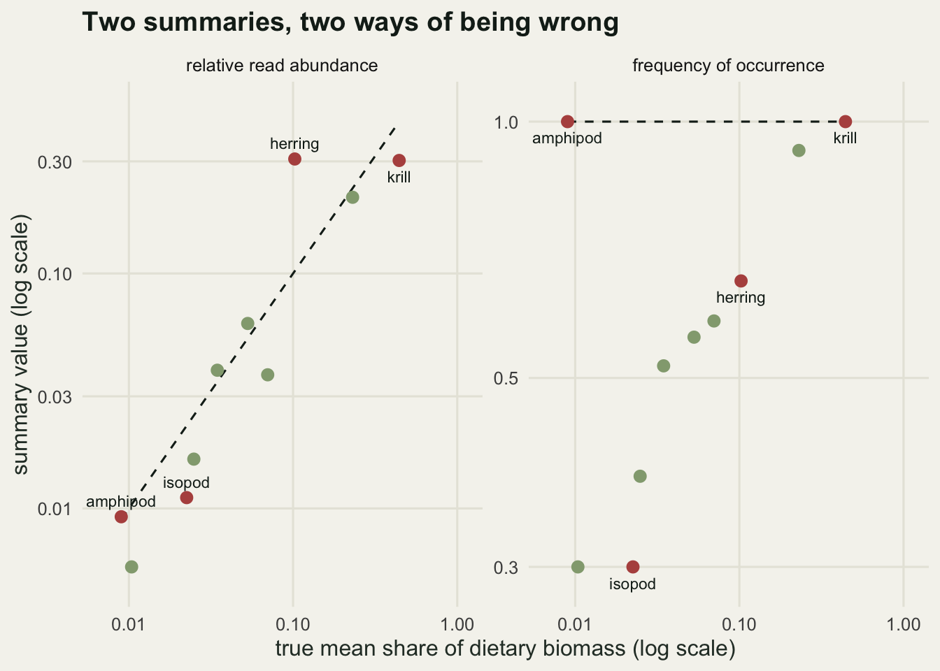

Figure 2: True mean share of dietary biomass against relative read abundance (left, with the one to one line) and against frequency of occurrence (right, with the ceiling at one). RRA scatters around the truth by the recovery factors; FOO runs into its ceiling.

Scoring RRA, POO and weighted POO

Percentage of occurrence is FOO rescaled so that the taxa sum to one, which puts it on the same scale as RRA. Weighted POO goes one step further: each sample carries a total weight of one, shared equally among the taxa detected in it, and the weights are averaged over samples. A taxon found alone in a gut earns a full unit from that gut; a taxon found alongside nine others earns a tenth.

poo <- foo / sum(foo)
wpoo <- colMeans(detected / rowSums(detected))
score <- data.frame(true_share = round(mean_w, 4), rra = round(mean_rra, 4),
                    poo = round(poo, 4), wpoo = round(wpoo, 4))
print(score)

           true_share    rra    poo   wpoo
krill          0.4428 0.3027 0.1609 0.1682
sandeel        0.2304 0.2110 0.1488 0.1531
herring        0.1024 0.3071 0.1046 0.1003
polychaete     0.0701 0.0370 0.0938 0.0916
shrimp         0.0529 0.0613 0.0898 0.0881
mysid          0.0346 0.0387 0.0831 0.0808
squid          0.0249 0.0162 0.0617 0.0579
amphipod       0.0090 0.0092 0.1609 0.1682
isopod         0.0225 0.0111 0.0483 0.0442
copepod        0.0104 0.0056 0.0483 0.0476

mae_all <- c(rra = mean(abs(mean_rra - mean_w)), poo = mean(abs(poo - mean_w)),
             wpoo = mean(abs(wpoo - mean_w)))
rho_all <- c(rra = cor(mean_rra, mean_w, method = "spearman"),
             poo = cor(poo, mean_w, method = "spearman"),
             wpoo = cor(wpoo, mean_w, method = "spearman"))
cat("mean absolute error on the proportion scale:\n")

mean absolute error on the proportion scale:

print(round(mae_all, 4))

   rra    poo   wpoo 
0.0435 0.0727 0.0708 

cat("rank correlation with true dietary biomass:\n")

rank correlation with true dietary biomass:

print(round(rho_all, 3))

  rra   poo  wpoo 
0.915 0.506 0.498 

On both criteria RRA wins, and it is not close. Its mean absolute error on the proportion scale is 0.0435 against 0.0727 for POO and 0.0708 for weighted POO, and its rank correlation with true dietary biomass is 0.915 against 0.506 and 0.498. That was not what I expected to write. The folklore is that occurrence based summaries are the safe choice, and measured against a known diet they are the least accurate of the three, on the ranking question as well as on the proportion question. Weighting POO by the number of taxa per sample changes almost nothing here, because the number of detected taxa varies little from gut to gut.

So why is FOO still worth reporting? Because accuracy against a diet you cannot see is not the only criterion. Change the marker, or the primer set, or the extraction protocol, and the recovery factors change with it. The following experiment redraws the recovery factors two hundred times, re-runs the sequencing each time, and watches how much each summary moves.

set.seed(11)
run_pipeline <- function(rec) {
  pb <- sweep(biomass, 2, rec / exp(mean(log(rec))), "*")
  pb <- pb / rowSums(pb)
  rb <- matrix(0L, n_samples, n_taxa)
  for (i in seq_len(n_samples)) {
    rb[i, ] <- as.integer(rmultinom(1, lib_size[i], pb[i, ]))
  }
  rb / rowSums(rb)
}
n_marker <- 200
rep_rra <- matrix(0, n_marker, n_taxa)
rep_poo <- matrix(0, n_marker, n_taxa)
rho_rra <- numeric(n_marker)
rho_poo <- numeric(n_marker)
for (b in seq_len(n_marker)) {
  rra_b <- run_pipeline(rlnorm(n_taxa, 0, 0.55) * rlnorm(n_taxa, 0, 0.35))
  foo_b <- colMeans(rra_b >= thr_base)
  rep_rra[b, ] <- colMeans(rra_b)
  rep_poo[b, ] <- foo_b / sum(foo_b)
  rho_rra[b] <- cor(colMeans(rra_b), mean_w, method = "spearman")
  rho_poo[b] <- cor(foo_b, mean_w, method = "spearman")
}
cat("markers simulated:", n_marker, "\n")

markers simulated: 200 

cat("mean per-taxon SD across markers, RRA", round(mean(apply(rep_rra, 2, sd)), 4),
    " POO", round(mean(apply(rep_poo, 2, sd)), 4), "\n")

mean per-taxon SD across markers, RRA 0.0475  POO 0.0019 

cat("ratio of those SDs:",
    round(mean(apply(rep_rra, 2, sd)) / mean(apply(rep_poo, 2, sd)), 1), "\n")

ratio of those SDs: 25.3 

cat("herring RRA across markers, 5th and 95th percentile:",
    round(quantile(rep_rra[, 3], 0.05), 3), round(quantile(rep_rra[, 3], 0.95), 3), "\n")

herring RRA across markers, 5th and 95th percentile: 0.033 0.216 

cat("herring POO across markers, 5th and 95th percentile:",
    round(quantile(rep_poo[, 3], 0.05), 3), round(quantile(rep_poo[, 3], 0.95), 3), "\n")

herring POO across markers, 5th and 95th percentile: 0.105 0.106 

cat("mean rank correlation with truth, RRA", round(mean(rho_rra), 3),
    " POO", round(mean(rho_poo), 3), "\n")

mean rank correlation with truth, RRA 0.901  POO 0.537 

Here is where occurrence earns its keep. Across markers, the mean standard deviation of a taxon’s estimate is 0.0495 for RRA and 0.0019 for POO, a ratio of 25.6. Herring’s RRA runs from 0.027 to 0.238 between the 5th and 95th percentile of markers, against a true share of 0.1024; its POO runs from 0.105 to 0.107. RRA still has the better mean rank correlation with the truth, 0.896 against 0.536, so on average it remains the better estimator of what the animals ate. What it is not is comparable. Two studies of the same population with different primer sets will report RRA values that differ by more than the diets they are describing, while their occurrence tables will agree.

The advantage also has a size, and it runs out. Sweeping the spread of the recovery factors from mild to severe shows where the two summaries change places.

set.seed(12)
sd_grid <- c(0.2, 0.4, 0.65, 0.9, 1.2, 1.5, 1.9)
n_bias <- 40
mae_rra <- numeric(length(sd_grid))
mae_poo <- numeric(length(sd_grid))
for (s in seq_along(sd_grid)) {
  acc_r <- numeric(n_bias)
  acc_p <- numeric(n_bias)
  for (b in seq_len(n_bias)) {
    rra_b <- run_pipeline(rlnorm(n_taxa, 0, sd_grid[s]))
    foo_b <- colMeans(rra_b >= thr_base)
    acc_r[b] <- mean(abs(colMeans(rra_b) - mean_w))
    acc_p[b] <- mean(abs(foo_b / sum(foo_b) - mean_w))
  }
  mae_rra[s] <- mean(acc_r)
  mae_poo[s] <- mean(acc_p)
}
spread_grid <- exp(2 * 1.645 * sd_grid)
print(round(data.frame(spread = spread_grid, rra = mae_rra, poo = mae_poo), 4))

    spread    rra    poo
1   1.9309 0.0113 0.0727
2   3.7285 0.0243 0.0727
3   8.4867 0.0346 0.0726
4  19.3173 0.0519 0.0718
5  51.8316 0.0646 0.0706
6 139.0731 0.0677 0.0698
7 518.5311 0.0893 0.0689

cross <- which(mae_rra > mae_poo)[1]
cat("RRA gives way to POO between recovery spreads of",
    round(spread_grid[cross - 1]), "and", round(spread_grid[cross]), "\n")

RRA gives way to POO between recovery spreads of 139 and 519 

cr_df <- rbind(
  data.frame(spread = spread_grid, mae = mae_rra, summ = "relative read abundance"),
  data.frame(spread = spread_grid, mae = mae_poo, summ = "percentage of occurrence"))
ggplot(cr_df, aes(spread, mae, colour = summ)) +
  geom_vline(xintercept = max(recovery) / min(recovery),
             colour = te_pal$line, linewidth = 0.9) +
  geom_line(linewidth = 1) +
  geom_point(size = 2.2) +
  scale_colour_manual(values = c("relative read abundance" = te_pal$clay,
                                 "percentage of occurrence" = te_pal$green),
                      name = NULL) +
  scale_x_log10() +
  labs(x = "spread of recovery factors, 5th to 95th percentile (log scale)",
       y = "mean absolute error", title = "Which summary is closer depends on the marker") +
  theme_te() + theme(legend.position = "bottom")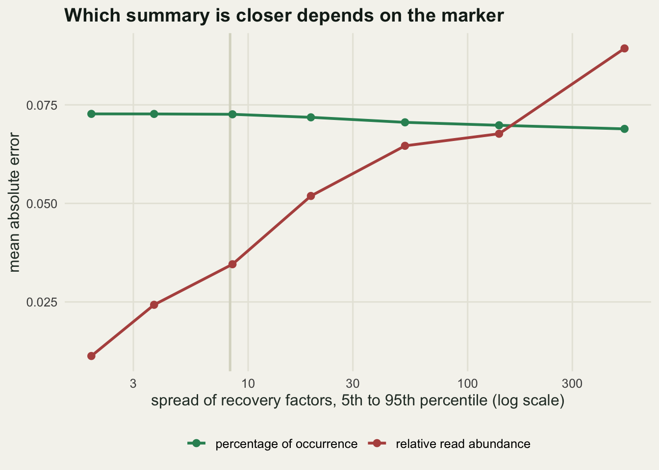

Figure 3: Mean absolute error against the true diet for relative read abundance and percentage of occurrence, as the spread of the recovery factors grows. The vertical line marks the spread used in the rest of the post.

RRA is the better estimate of dietary proportions while the recovery factors stay within roughly an order of magnitude of each other, and it gives way to occurrence somewhere between a spread of 52 and 139. A blocked or badly mismatched primer puts you on the wrong side of that crossing without any warning in the data, which is why the winner cannot be settled once and quoted as a rule. A ranking question and a proportion question are not the same question, and neither is the comparability question.

The detection threshold is a lever nobody reports

Every occurrence summary needs a rule for calling a taxon absent, and that rule is usually buried in the methods as a single sentence. It is not a detail. Sweep it, and FOO moves for some taxa and not for others.

thr_grid <- c(1e-5, 5e-5, 1e-4, 5e-4, 1e-3, 2e-3, 5e-3, 1e-2, 2e-2, 5e-2)
sweep_foo <- sapply(thr_grid, function(tt) colMeans(rra >= tt))
dimnames(sweep_foo) <- list(taxon_lab, format(thr_grid, scientific = FALSE))
print(round(sweep_foo, 3))

           0.00001 0.00005 0.00010 0.00050 0.00100 0.00200 0.00500 0.01000
krill        1.000   1.000   1.000   1.000   1.000   1.000   1.000   1.000
sandeel      0.925   0.925   0.925   0.925   0.925   0.925   0.925   0.925
herring      0.650   0.650   0.650   0.650   0.650   0.650   0.650   0.650
polychaete   0.583   0.583   0.583   0.583   0.583   0.583   0.583   0.583
shrimp       0.558   0.558   0.558   0.558   0.558   0.558   0.558   0.558
mysid        0.517   0.517   0.517   0.517   0.517   0.517   0.517   0.517
squid        0.383   0.383   0.383   0.383   0.383   0.383   0.383   0.367
amphipod     1.000   1.000   1.000   1.000   1.000   0.967   0.700   0.292
isopod       0.300   0.300   0.300   0.300   0.300   0.300   0.300   0.300
copepod      0.300   0.300   0.300   0.300   0.300   0.300   0.300   0.250
           0.02000 0.05000
krill        1.000   1.000
sandeel      0.925   0.892
herring      0.650   0.650
polychaete   0.500   0.250
shrimp       0.542   0.442
mysid        0.500   0.300
squid        0.283   0.133
amphipod     0.067   0.008
isopod       0.175   0.067
copepod      0.117   0.000

cat("amphipod FOO at 0.1 percent and at 1 percent:",
    round(sweep_foo["amphipod", 5], 3), round(sweep_foo["amphipod", 8], 3), "\n")

amphipod FOO at 0.1 percent and at 1 percent: 1 0.292 

cat("herring FOO at 0.1 percent and at 1 percent:",
    round(sweep_foo["herring", 5], 3), round(sweep_foo["herring", 8], 3), "\n")

herring FOO at 0.1 percent and at 1 percent: 0.65 0.65 

cat("copepod FOO at 0.1 percent and at 1 percent:",
    round(sweep_foo["copepod", 5], 3), round(sweep_foo["copepod", 8], 3), "\n")

copepod FOO at 0.1 percent and at 1 percent: 0.3 0.25 

Two thresholds in common use are 0.1 percent and 1 percent of a sample’s reads. At 0.1 percent the amphipod, which every animal ate in trace amounts, has a FOO of 1 and herring, eaten in bulk by fewer animals, has 0.65. At 1 percent the amphipod has 0.3 and herring is unchanged at 0.65. The rare but widespread taxon has lost seven tenths of its occurrence and the common but patchy taxon has lost none.

I had expected to report the two moving in opposite directions. They cannot: FOO is a count of samples above a threshold, so raising the threshold can only push it down or leave it alone, for every taxon. What moves in opposite directions is their ranking. At the lower threshold the amphipod ties krill as the most frequently recorded prey and herring is fourth; at the higher threshold the amphipod has dropped to eighth of the ten and herring has not moved. Nothing about the animals changed between those two sentences.

sw_df <- data.frame(threshold = rep(thr_grid, each = n_taxa),
                    foo = as.vector(sweep_foo),
                    taxon = rep(taxon_lab, times = length(thr_grid)))
sw_df$grp <- ifelse(sw_df$taxon == "amphipod", "amphipod: every gut, trace amounts",
             ifelse(sw_df$taxon == "herring", "herring: fewer guts, in bulk", "other prey"))
ggplot(sw_df, aes(threshold, foo, group = taxon, colour = grp)) +
  geom_vline(xintercept = c(0.001, 0.01), colour = te_pal$line, linewidth = 0.9) +
  geom_line(linewidth = 0.9) +
  scale_colour_manual(values = c("amphipod: every gut, trace amounts" = te_pal$clay,
                                 "herring: fewer guts, in bulk" = te_pal$green,
                                 "other prey" = te_pal$sage), name = NULL) +
  scale_x_log10() +
  labs(x = "detection threshold (share of the sample's reads, log scale)",
       y = "frequency of occurrence", title = "The threshold reorders the diet") +
  theme_te() +
  theme(legend.position = "bottom") +
  guides(colour = guide_legend(nrow = 2))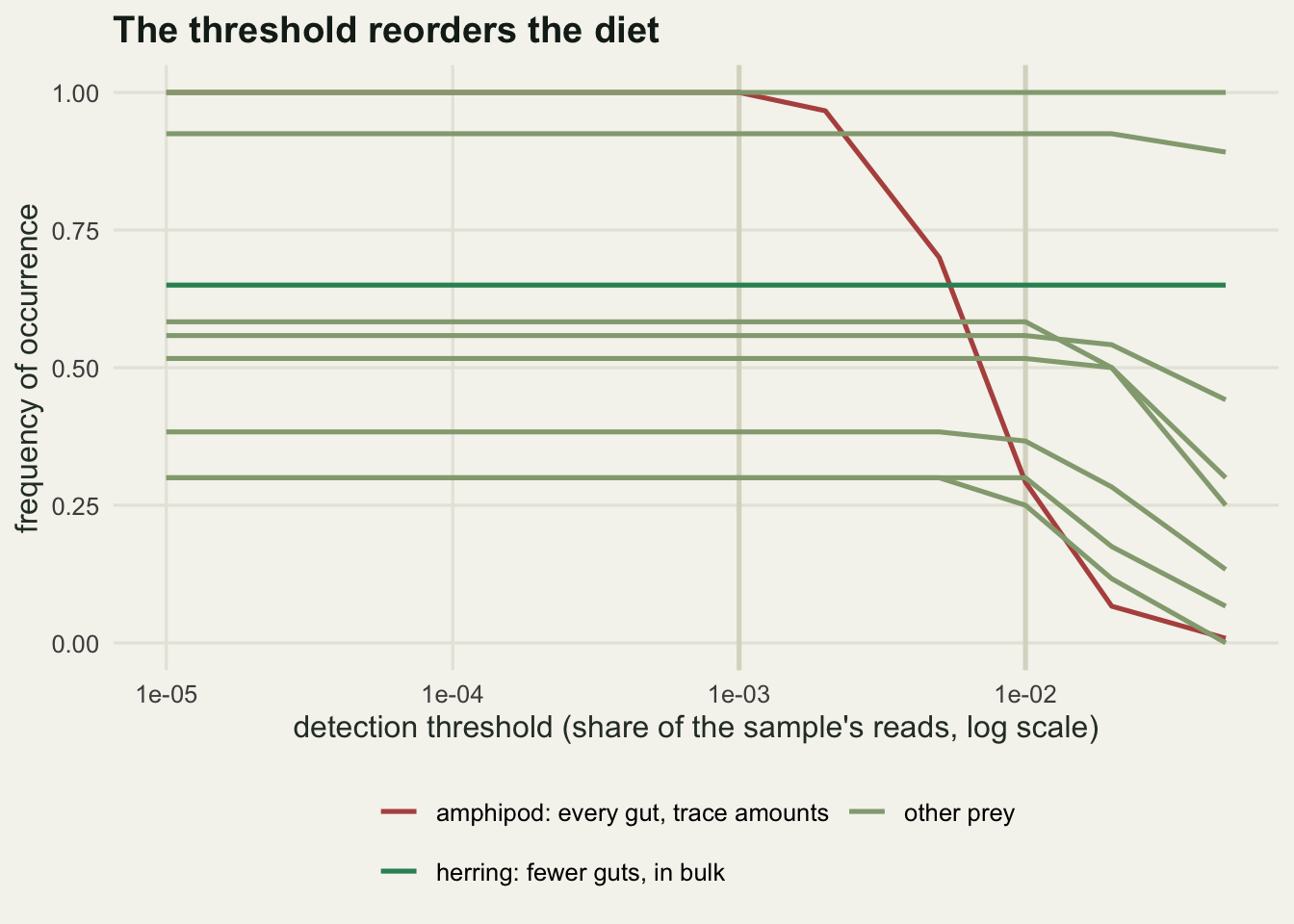

Figure 4: Frequency of occurrence against the detection threshold for all ten prey taxa. The two vertical lines mark thresholds of 0.1 percent and 1 percent of a sample’s reads.

A threshold also decides how much of the contamination and tag jumping in a run survives into the results, which is a second reason to set it deliberately rather than by habit. That is the subject of the third tutorial in this cluster.

What none of these summaries can give you

None of RRA, FOO, POO or weighted POO recovers consumed biomass, and no amount of care with the bioinformatics changes that. The recovery factors are properties of the marker, the tissue and the protocol rather than of the diet, and nothing inside the read table identifies them. In this simulation I knew them because I chose them; with real faeces they are estimable only from control mixtures of known composition run through the same pipeline, and those corrections transfer poorly to prey and digestive states the controls did not include.

The row totals are the second thing gone for good. A read table cannot tell you whether an animal ate a little or a lot, so any per animal intake or population level total needs the quantity to come from outside the sequencer: gut fullness, meal mass, energetics.

The reporting standard that follows is unglamorous. Give both summaries, with the detection threshold stated as a number, and let the ecological question pick which one carries the argument. FOO answers “what does this population eat”, and it answers it well: presence was recovered exactly here across an eightfold spread of recovery factors. RRA answers “what does this individual eat most of”, offsets and all, so its differences between taxa are worth less than its differences within a taxon across animals or seasons. Neither answers “how much”, and a paper that reports one summary alone has made that choice for its readers silently.

Where to go next

The recovery factors here were one number per taxon, which hides most of what a PCR does: efficiency differences compound over cycles, so a small per cycle advantage becomes a large one after thirty five of them, and the bias depends on the starting mixture. The next tutorial in this cluster, on PCR bias and amplification efficiency, builds the cycle by cycle model and measures how far compounding can carry a read proportion away from the template proportion.

References

Deagle BE, Thomas AC, McInnes JC, Clarke LJ, Vesterinen EJ, Clare EL, Kartzinel TR, Eveson JP 2019 Molecular Ecology 28(2):391-406 (10.1111/mec.14734)

Deagle BE, Thomas AC, Shaffer AK, Trites AW, Jarman SN 2013 Molecular Ecology Resources 13(4):620-633 (10.1111/1755-0998.12103)

Pompanon F, Deagle BE, Symondson WOC, Brown DS, Jarman SN, Taberlet P 2012 Molecular Ecology 21(8):1931-1950 (10.1111/j.1365-294X.2011.05403.x)

Gloor GB, Macklaim JM, Pawlowsky-Glahn V, Egozcue JJ 2017 Frontiers in Microbiology 8:2224 (10.3389/fmicb.2017.02224)

Aitchison J 1986 The Statistical Analysis of Compositional Data. Chapman and Hall, ISBN 978-0-412-28060-3

Related tutorials

• PCR bias and amplification efficiency
• Contamination filtering in metabarcoding
• Checking a metabarcoding analysis
• Log-ratio transformations: clr, alr and ilr