PCR bias and amplification efficiency

Simulating taxon-specific PCR efficiency in R: why metabarcoding bias is linear in the log-ratio, what a mock community corrects, and where the mock fails.

A diet study extracts DNA from a faecal sample, amplifies a barcode marker, sequences the product and gets a table of read counts. The question the study actually wants to answer is how much of each prey item the animal ate. Between those two things sits a chain of steps, and one of them does most of the damage.

The sibling post Metabarcoding reads as compositional data establishes the frame this one works inside: a read table carries no total, so only ratios between taxa are interpretable, and each taxon arrives at the sequencer multiplied by its own recovery factor. That post takes the recovery factor as given. This one takes it apart. The largest single contributor is taxon-specific amplification efficiency: some templates copy more readily than others under the same primer pair, and PCR compounds the difference once per cycle. The log-ratio machinery that makes this tractable was built in Log-ratio transformations: CLR and ILR and is used here without re-derivation.

The plan is to derive the bias from the amplification process, then measure it against a simulator that copies molecules one cycle at a time rather than applying a single closed-form factor. What gets measured: whether the simulated drift matches the algebra, how large the error becomes at ordinary cycle numbers, what a plateauing reaction does to it, how well a mock community of known composition removes it, what that correction costs in variance, and how the whole thing ranks against the other places a run loses its quantitative meaning. Everything is base R plus ggplot2.

library(ggplot2)

te_pal <- list(forest = "#275139", green = "#2f8f63", sage = "#93a87f",
               clay = "#b5534e", gold = "#cda23f", line = "#dad9ca",
               ink = "#16241d", paper = "#f5f4ee")

theme_te <- function() {
  theme_minimal(base_size = 12) +
    theme(panel.grid.minor = element_blank(),
          panel.grid.major = element_line(colour = "#e7e6dc"),
          plot.background = element_rect(fill = "#f5f4ee", colour = NA),
          panel.background = element_rect(fill = "#f5f4ee", colour = NA),
          plot.title = element_text(face = "bold", colour = te_pal$ink),
          axis.title = element_text(colour = "#2c3a31"))
}

The bias is linear in the log-ratio

Write the per-cycle efficiency of a taxon as the probability that any given template molecule is copied in a cycle. If that probability is e and there are N0 molecules to start with, then after n cycles the expected count is N0 * (1 + e)^n. Two taxa with efficiencies e1 and e2 therefore end the reaction with a ratio equal to their starting ratio multiplied by ((1 + e1) / (1 + e2))^n. Taking logs turns that into a statement worth keeping:

the observed log-ratio equals the true log-ratio plus n * log((1 + e1) / (1 + e2)).

The distortion is additive on the log-ratio scale, proportional to the cycle number, and independent of the starting composition. That is why log-ratios are the right coordinates for this problem and not a stylistic preference: on that scale the bias is a constant offset, and a constant offset can be subtracted.

The simulator below does not use the closed form. It copies molecules. Each cycle, every template either replicates or does not, with probability equal to the taxon’s efficiency, so the count gained is a binomial draw. That keeps the process stochastic in the way real PCR is stochastic, which matters most in the first few cycles when molecule counts are small. Once a taxon passes ten million molecules the binomial is replaced by its normal approximation, both because rbinom will not accept sizes that large and because the relative sampling noise by then is far below anything else in the run.

mol_switch <- 1e7

pcr_step <- function(n_mol, p_dup) {
  gained <- numeric(length(n_mol))
  small <- n_mol < mol_switch
  if (any(small)) {
    gained[small] <- rbinom(sum(small), round(n_mol[small]), p_dup[small])
  }
  if (any(!small)) {
    mu_add <- n_mol[!small] * p_dup[!small]
    sd_add <- sqrt(n_mol[!small] * p_dup[!small] * (1 - p_dup[!small]))
    gained[!small] <- pmax(0, round(mu_add + sd_add * rnorm(sum(!small))))
  }
  n_mol + gained
}

pcr_run <- function(n0, eff, n_cycles, capacity = Inf) {
  n_mol <- n0
  for (cyc in seq_len(n_cycles)) {
    fade <- if (is.finite(capacity)) max(0, 1 - sum(n_mol) / capacity) else 1
    n_mol <- pcr_step(n_mol, eff * fade)
  }
  n_mol
}

cap_k <- 1e12
print(c(exact_binomial_below = mol_switch, plateau_capacity = cap_k))

exact_binomial_below     plateau_capacity 
               1e+07                1e+12 

The capacity argument is the plateau term and is switched off for now. The calibration run uses two taxa whose efficiencies differ by a realistic amount, starts them at equal template counts so the true log-ratio is zero, and compares the realised drift after thirty cycles against the closed form.

set.seed(20260817)
eff_pair <- c(0.90, 0.75)
n0_pair <- c(5000, 5000)
cyc_ref <- 30L
n_rep <- 200L
print(c(eff_fast = eff_pair[1], eff_slow = eff_pair[2],
        templates_each = n0_pair[1], cycles = cyc_ref, replicates = n_rep))

      eff_fast       eff_slow templates_each         cycles     replicates 
          0.90           0.75        5000.00          30.00         200.00 

log_gap <- function(x) log(x[1] / x[2])
drift_obs <- replicate(n_rep, log_gap(pcr_run(n0_pair, eff_pair, cyc_ref)) - log_gap(n0_pair))
drift_pred <- cyc_ref * log((1 + eff_pair[1]) / (1 + eff_pair[2]))
print(round(c(simulated = mean(drift_obs), closed_form = drift_pred,
              mc_se = sd(drift_obs) / sqrt(n_rep), sd_across_runs = sd(drift_obs),
              fold_simulated = exp(mean(drift_obs)), fold_closed = exp(drift_pred)), 4))

     simulated    closed_form          mc_se sd_across_runs fold_simulated 
        2.4672         2.4671         0.0004         0.0060        11.7895 
   fold_closed 
       11.7887 

The simulated drift is 2.4672 and the algebra says 2.4671, a difference well inside the Monte Carlo standard error of 0.0004. On the fold scale that is 11.7895 against 11.7887. So the molecule-by-molecule process and the closed form describe the same thing, and the closed form can be used for the parts of the argument where speed matters.

The second number in that block deserves attention. The standard deviation of the drift across replicate reactions is 0.0060, which is tiny. PCR is a stochastic process, but starting from five thousand template copies the stochasticity contributes almost nothing to the final log-ratio. The bias is nearly deterministic. That is bad news and good news at once: bad, because replicating the PCR does not average the problem away; good, because a deterministic offset is exactly the kind of thing a calibration can remove.

How large the error gets

Thirty cycles turned a fifteen-point efficiency difference into a twelvefold error in the estimated ratio. The compounding is worth seeing across the cycle numbers people actually run.

cyc_grid <- c(25, 30, 35, 40)
fold_gap <- exp(cyc_grid * log((1 + eff_pair[1]) / (1 + eff_pair[2])))
print(round(setNames(fold_gap, paste0("cycles_", cyc_grid)), 3))

cycles_25 cycles_30 cycles_35 cycles_40 
    7.814    11.789    17.785    26.830 

cyc_std <- 35
eff_base <- 0.80
delta_for <- function(target) (1 + eff_base) * target^(1 / cyc_std) - 1 - eff_base
print(round(c(cycles = cyc_std, base_efficiency = eff_base,
              delta_twofold = delta_for(2), delta_tenfold = delta_for(10)), 4))

         cycles base_efficiency   delta_twofold   delta_tenfold 
        35.0000          0.8000          0.0360          0.1224 

At 25 cycles the ratio is out by 7.814-fold, at 30 by 11.789, at 35 by 17.785 and at 40 by 26.830. Running five more cycles because a sample was low-yield is not a neutral act.

The second block inverts the question. Against a baseline efficiency of 0.8 and 35 cycles, a per-cycle efficiency difference of 0.0360 is enough to double the estimated ratio of two taxa, and a difference of 0.1224 multiplies it by ten. A per-cycle efficiency gap of three and a half percentage points is not something a primer-design check would flag, and it sits well inside the range that primer mismatch and template secondary structure produce routinely.

delta_grid <- c(0.02, 0.05, 0.10, 0.15)
grid_dat <- expand.grid(cycle = 0:45, delta = delta_grid)
grid_dat$fold <- exp(grid_dat$cycle *
                     log((1 + eff_base + grid_dat$delta) / (1 + eff_base)))
grid_dat$gap <- factor(sprintf("%.2f", grid_dat$delta))

p_fold <- ggplot(grid_dat, aes(cycle, fold, colour = gap)) +
  geom_hline(yintercept = c(2, 10), linetype = 2, colour = te_pal$ink,
             linewidth = 0.4) +
  geom_line(linewidth = 0.8) +
  scale_y_log10() +
  scale_colour_manual(values = c("0.02" = te_pal$sage, "0.05" = te_pal$green,
                                 "0.10" = te_pal$gold, "0.15" = te_pal$clay)) +
  labs(title = "A small per-cycle gap is a large error by cycle 35",
       x = "PCR cycles", y = "fold error in the estimated ratio",
       colour = "efficiency gap") +
  theme_te() + theme(legend.position = "top")
p_fold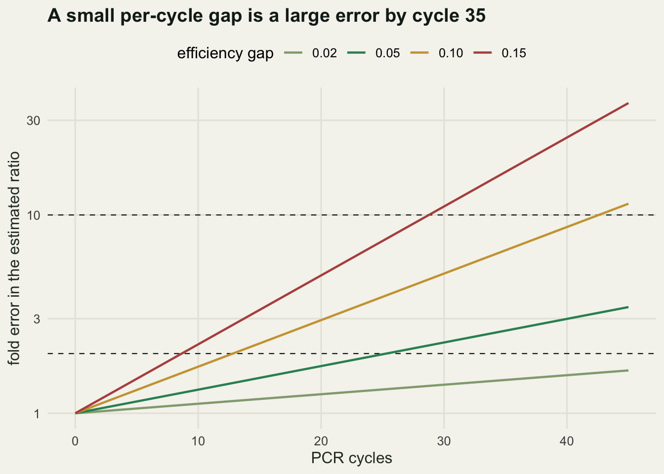

Figure 1: Fold error in an estimated ratio of two taxa as a function of cycle number, for four per-cycle efficiency gaps against a baseline efficiency of 0.8. Dashed lines mark a twofold and a tenfold error.

The plateau changes the shape of the problem

Nothing above is true of a real reaction past a certain point. Primers, nucleotides and polymerase run out, and the efficiency falls. The standard picture of a plateau is a total product ceiling, so the simplest honest version of it multiplies every taxon’s efficiency by a factor that declines linearly with the total amount of product already made and reaches zero at a capacity. That is the capacity argument already in pcr_run, set here to 1e12 amplicons, which is the right order for a small-volume reaction.

The capacity term does not act on taxa differentially. It scales every efficiency by the same factor. That looks as though it should leave the bias alone, and it does not, because the bias per cycle depends on the ratio of 1 + e1 to 1 + e2, and as the efficiencies are driven toward zero that ratio is driven toward one. Once the reaction plateaus, the bias stops accumulating.

set.seed(20260818)
n_rep_sat <- 60L
print(c(replicates_per_cell = n_rep_sat, capacity = cap_k))

replicates_per_cell            capacity 
              6e+01               1e+12 

sat_tab <- t(sapply(cyc_grid, function(nc) {
  free <- replicate(n_rep_sat, log_gap(pcr_run(n0_pair, eff_pair, nc)) - log_gap(n0_pair))
  satd <- replicate(n_rep_sat,
                    log_gap(pcr_run(n0_pair, eff_pair, nc, cap_k)) - log_gap(n0_pair))
  c(cycles = nc, free_lr = mean(free), plateau_lr = mean(satd),
    free_fold = exp(mean(free)), plateau_fold = exp(mean(satd)))
}))
print(round(sat_tab, 3))

     cycles free_lr plateau_lr free_fold plateau_fold
[1,]     25   2.056      2.053     7.815        7.791
[2,]     30   2.468      2.407    11.796       11.097
[3,]     35   2.879      2.463    17.790       11.735
[4,]     40   3.290      2.463    26.841       11.743

At 25 cycles the reaction has not yet noticed the ceiling and the two columns agree: 7.815 against 7.791. By 40 cycles the unconstrained reaction is out by 26.841-fold and the plateauing one by 11.743. So the plateau partly rescues the measurement, and it does so by freezing the bias at whatever value it had reached when the reagents started to run short. Between 35 and 40 cycles the plateau column barely moves at all, from 11.735 to 11.743.

That is the first measured surprise, and it inverts a piece of common advice. Cutting the cycle number from 40 to 35 does nothing for a reaction that plateaus at either, because the bias was locked in around cycle 30. What sets the bias is not how many cycles were run but how many cycles the reaction spent growing freely before it hit the ceiling, and that is set by how much template went in.

traj <- t(sapply(0:40, function(nc) {
  free <- if (nc == 0) 0 else
    mean(replicate(20, log_gap(pcr_run(n0_pair, eff_pair, nc)) - log_gap(n0_pair)))
  satd <- if (nc == 0) 0 else
    mean(replicate(20, log_gap(pcr_run(n0_pair, eff_pair, nc, cap_k)) - log_gap(n0_pair)))
  c(cycle = nc, free = free, plateau = satd)
}))
traj_long <- rbind(
  data.frame(cycle = traj[, "cycle"], lr = traj[, "free"], reaction = "no ceiling"),
  data.frame(cycle = traj[, "cycle"], lr = traj[, "plateau"], reaction = "plateau at 1e12"))

p_plateau <- ggplot(traj_long, aes(cycle, lr, colour = reaction)) +
  geom_line(linewidth = 0.9) +
  scale_colour_manual(values = c("no ceiling" = te_pal$clay,
                                 "plateau at 1e12" = te_pal$forest)) +
  labs(title = "The plateau freezes the bias where it stands",
       x = "PCR cycles", y = "log-ratio bias", colour = NULL) +
  theme_te() + theme(legend.position = "top")
p_plateau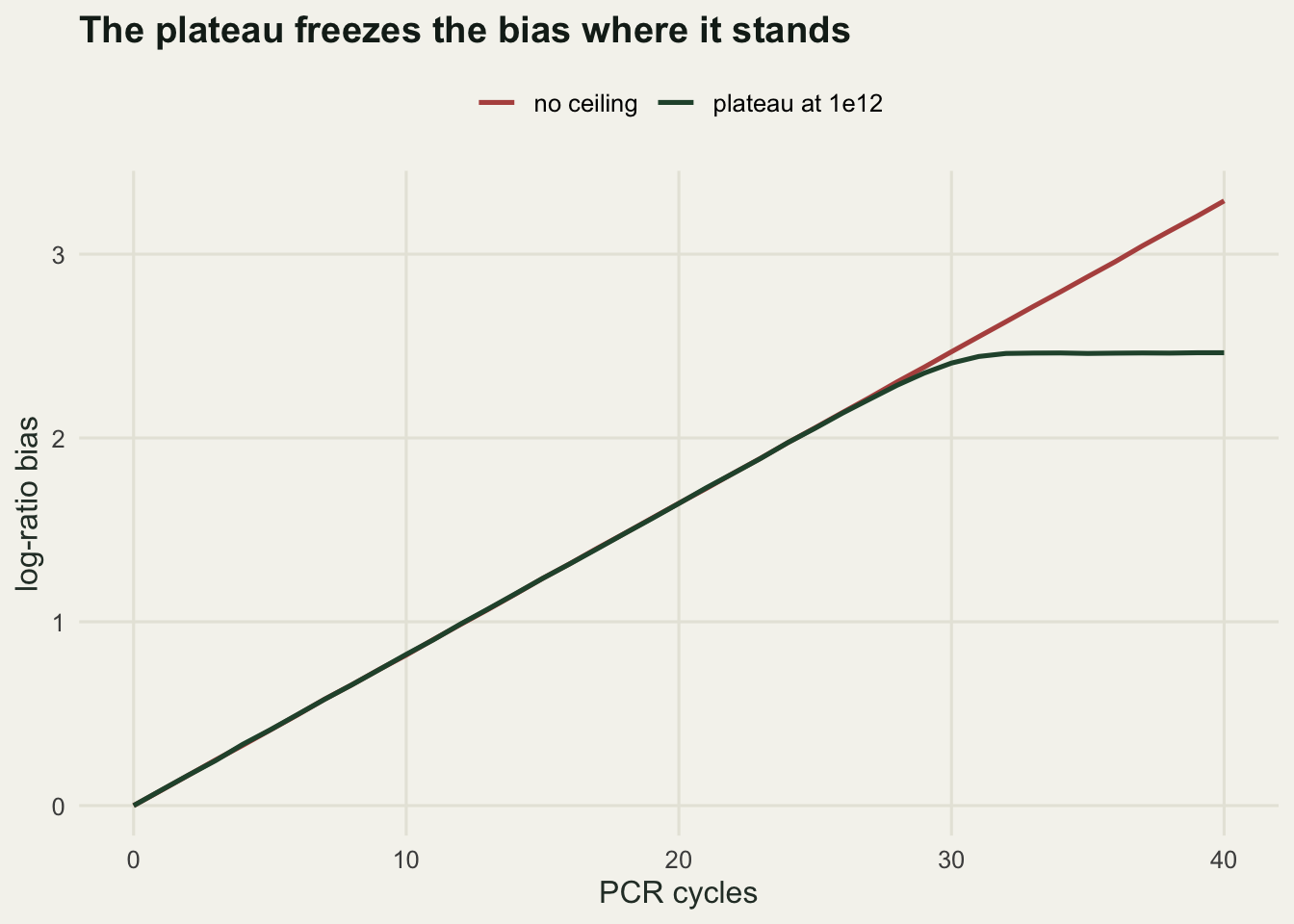

Figure 2: Log-ratio bias against cycle number for two taxa with efficiencies 0.9 and 0.75, with and without a product ceiling at 1e12 amplicons. The unconstrained trace is a straight line; the plateauing trace bends over and stops.

The awkward consequence is that the bias is no longer a property of the primer pair and the cycle number alone. It now depends on the sample. The block below runs the same pair of taxa at 35 cycles with a ceiling, changing only how much of the starting template belongs to the efficient taxon.

start_frac <- c(0.50, 0.20, 0.05)
comp_tab <- t(sapply(start_frac, function(fr) {
  n0v <- c(10000 * fr, 10000 * (1 - fr))
  b <- replicate(n_rep_sat, log_gap(pcr_run(n0v, eff_pair, cyc_std, cap_k)) - log_gap(n0v))
  c(start_share_fast = fr, plateau_lr = mean(b), plateau_fold = exp(mean(b)))
}))
print(round(comp_tab, 3))

     start_share_fast plateau_lr plateau_fold
[1,]             0.50      2.462       11.730
[2,]             0.20      2.557       12.895
[3,]             0.05      2.662       14.320

print(round(c(spread_in_fitted_factor =
                exp(max(comp_tab[, "plateau_lr"]) - min(comp_tab[, "plateau_lr"]))), 3))

spread_in_fitted_factor 
                  1.221 

The correction factor a calibration would fit is 11.730-fold when the efficient taxon starts at half the template, 12.895 when it starts at a fifth and 14.320 when it starts at a twentieth: a spread of 1.221 across starting compositions that a real sample set would span easily. The bias is still nearly deterministic; it is just no longer the same constant for every sample.

What a mock community recovers

The practical answer to a fixed multiplicative bias is a mock community: a mixture of known composition, built from the target taxa, taken through the same protocol as the samples. If the observed log-ratios in the mock differ from the known ones by a constant offset, that offset is the bias, and subtracting it from the samples removes it. In centred log-ratio coordinates the estimator is one line.

set.seed(20260819)
eff_tax <- c(0.92, 0.88, 0.84, 0.80, 0.76, 0.72)
n_taxa <- length(eff_tax)
tax_lab <- paste0("taxon ", seq_len(n_taxa))
depth_reads <- 50000L
load_std <- 30000
n_rep_mock <- 200L
p_mock <- rep(1 / n_taxa, n_taxa)
p_field <- c(0.20, 0.19, 0.18, 0.16, 0.14, 0.13)
p_skew <- c(0.80, 0.10, 0.04, 0.03, 0.02, 0.01)
print(c(taxa = n_taxa, reads_per_sample = depth_reads, templates_in = load_std,
        cycles = cyc_std, runs_per_scenario = n_rep_mock))

             taxa  reads_per_sample      templates_in            cycles 
                6             50000             30000                35 
runs_per_scenario 
              200 

print(round(setNames(eff_tax, tax_lab), 2))

taxon 1 taxon 2 taxon 3 taxon 4 taxon 5 taxon 6 
   0.92    0.88    0.84    0.80    0.76    0.72 

clr_of <- function(p) log(p) - mean(log(p))
amplify_seq <- function(p0, total0, n_cycles = cyc_std, capacity = cap_k) {
  n_mol <- pcr_run(p0 * total0, eff_tax, n_cycles, capacity)
  reads <- as.numeric(rmultinom(1, depth_reads, n_mol / sum(n_mol)))
  reads / sum(reads)
}

mock_obs <- replicate(n_rep_mock, amplify_seq(p_mock, load_std))
bias_hat <- rowMeans(apply(mock_obs, 2, clr_of)) - clr_of(p_mock)
bias_free <- cyc_std * (log(1 + eff_tax) - mean(log(1 + eff_tax)))
print(round(rbind(mock_estimate = bias_hat, free_pcr_theory = bias_free), 4))

                  [,1]   [,2]   [,3]    [,4]    [,5]    [,6]
mock_estimate   1.5420 0.9407 0.3321 -0.2949 -0.9317 -1.5882
free_pcr_theory 1.8968 1.1599 0.4072 -0.3621 -1.1486 -1.9532

Six taxa with per-cycle efficiencies from 0.92 down to 0.72, an even mock, 50000 reads per sample and 35 cycles. The estimated bias vector runs from 1.542 for the most efficient taxon to -1.5882 for the least. The free-PCR theory says it should run from 1.8968 to -1.9532. The mock measures something smaller than the theory, and the reason is the plateau: the reaction stopped accumulating bias before cycle 35.

That gap has a consequence for anyone who wants efficiencies rather than a correction. Only ratios of 1 + e are identifiable from a mock, so the recovery below anchors on the first taxon’s true efficiency and reads off the rest.

eff_rec <- exp(log(1 + eff_tax[1]) + (bias_hat - bias_hat[1]) / cyc_std) - 1
print(round(rbind(recovered = eff_rec, truth = eff_tax), 4))

          [,1]   [,2]   [,3]   [,4]  [,5]   [,6]
recovered 0.92 0.8873 0.8548 0.8218 0.789 0.7557
truth     0.92 0.8800 0.8400 0.8000 0.760 0.7200

print(round(c(max_abs_efficiency_error = max(abs(eff_rec - eff_tax))), 4))

max_abs_efficiency_error 
                  0.0357 

The recovered efficiencies are compressed toward the anchor: 0.7557 for the last taxon against a truth of 0.72, with a worst error of 0.0357 across the six. Anyone reporting per-cycle efficiencies from a plateauing mock is reporting numbers that are too similar to each other. The correction itself does not care, because it applies the measured offset directly and never converts it into an efficiency.

clr_mean <- function(p0, total0, n_cycles = cyc_std) {
  rowMeans(apply(replicate(n_rep_mock, amplify_seq(p0, total0, n_cycles)), 2, clr_of))
}
samp_clr <- apply(replicate(n_rep_mock, amplify_seq(p_field, load_std)), 2, clr_of)
scen <- list(matched = list(rowMeans(samp_clr), p_field),
             skewed = list(clr_mean(p_skew, load_std), p_skew),
             tenfold_less = list(clr_mean(p_field, load_std / 10), p_field),
             hundredfold_less = list(clr_mean(p_field, load_std / 100), p_field),
             forty_cycles = list(clr_mean(p_field, load_std, 40), p_field))
resid_tab <- t(sapply(scen, function(s) {
  raw <- s[[1]] - clr_of(s[[2]])
  fixed <- raw - bias_hat
  c(uncorrected = sqrt(mean(raw^2)), corrected = sqrt(mean(fixed^2)),
    worst_taxon = max(abs(fixed)), worst_fold = exp(max(abs(fixed))))
}))
print(round(resid_tab, 4))

                 uncorrected corrected worst_taxon worst_fold
matched               1.0598    0.0088      0.0134     1.0135
skewed                1.0201    0.0486      0.0717     1.0744
tenfold_less          1.1980    0.1295      0.1935     1.2135
hundredfold_less      1.2940    0.2255      0.3312     1.3927
forty_cycles          1.0612    0.0075      0.0132     1.0133

For a sample whose composition and template load resemble the mock, the correction works almost perfectly: the root mean square log-ratio error falls from 1.0598 to 0.0088, and the worst taxon is out by a factor of 1.0135. That is the advertised behaviour.

Then the two failure modes. A sample dominated by one taxon at 80 percent, run at the same template load, leaves a residual of 0.0486 with a worst taxon at 1.0744-fold. Cutting the template input tenfold leaves 0.1295 with a worst taxon at 1.2135-fold, and a hundredfold cut leaves 0.2255 and 1.3927-fold. Running the sample for 40 cycles instead of 35 leaves 0.0075, which is no worse than the matched case at all.

The ordering there is not the obvious one. A cycle-number mismatch between mock and sample costs nothing once both reactions plateau, a composition mismatch costs a little, and a template-load mismatch costs an order of magnitude more than either. The thing to standardise between a mock and a sample set is the amount of DNA going in, and that is the one thing most protocols leave to whatever the extraction happened to yield.

A taxon the mock does not contain

The second failure is sharper. A mock is built from the taxa somebody thought to include. A faecal sample contains what the animal ate. When a taxon in the sample has no counterpart in the mock, it has no correction factor, and the usual practice is to leave it alone.

sub_clr <- function(p) {
  q <- p[1:5] / sum(p[1:5])
  log(q) - mean(log(q))
}
bias5 <- rowMeans(apply(mock_obs, 2, sub_clr)) - sub_clr(p_mock)
offset5 <- c(bias5, 0)
offset5 <- offset5 - mean(offset5)
err_none <- rowMeans(samp_clr) - clr_of(p_field)
err_full <- rowMeans(samp_clr - bias_hat) - clr_of(p_field)
err_miss <- rowMeans(samp_clr - offset5) - clr_of(p_field)
print(round(rbind(no_correction = err_none, full_mock = err_full,
                  mock_missing_taxon6 = err_miss), 4))

                       [,1]    [,2]    [,3]    [,4]    [,5]    [,6]
no_correction        1.5298  0.9347  0.3265 -0.2926 -0.9237 -1.5747
full_mock           -0.0122 -0.0060 -0.0056  0.0024  0.0079  0.0134
mock_missing_taxon6  0.3055  0.3116  0.3120  0.3200  0.3256 -1.5747

print(round(c(rms_full_mock = sqrt(mean(err_full^2)),
              rms_missing = sqrt(mean(err_miss^2)),
              error_on_missing_taxon = err_miss[6],
              fold_on_missing_taxon = exp(abs(err_miss[6])),
              spillover_on_the_others = mean(err_miss[1:5]),
              spillover_fold = exp(mean(err_miss[1:5])),
              rms_ratio = sqrt(mean(err_miss^2)) / sqrt(mean(err_full^2))), 4))

          rms_full_mock             rms_missing  error_on_missing_taxon 
                 0.0088                  0.7043                 -1.5747 
  fold_on_missing_taxon spillover_on_the_others          spillover_fold 
                 4.8295                  0.3149                  1.3702 
              rms_ratio 
                80.0799 

The uncorrected taxon keeps its full error of -1.5747 in log-ratio units, a 4.8295-fold underestimate. That is expected. What is not expected on first sight is the second row of numbers: the five taxa that were corrected are now all wrong in the same direction, by 0.3149 on average, a 1.3702-fold overestimate each. The root mean square error over all six taxa is 0.7043 against 0.0088 for the complete mock, a degradation by a factor of 80.0799 caused by one absent reference.

The mechanism is the closure. A centred log-ratio is measured against the geometric mean of the whole composition, so one taxon left at the wrong value drags the reference point and every other taxon moves with it. An incomplete mock does not simply fail to correct the taxa it lacks; it damages the taxa it does correct. The defensible choice is to drop the uncovered taxon from the composition and analyse the sub-composition, which log-ratio coordinates permit and proportions do not.

err_low10 <- clr_mean(p_field, load_std / 10) - clr_of(p_field) - bias_hat
err_dat <- do.call(rbind, lapply(
  list(list("no correction", err_none), list("mock, matched sample", err_full),
       list("mock, tenfold less template", err_low10),
       list("mock missing taxon 6", err_miss)),
  function(s) data.frame(scenario = s[[1]], taxon = tax_lab, err = s[[2]])))
err_dat$scenario <- factor(err_dat$scenario,
                           c("no correction", "mock, matched sample",
                             "mock, tenfold less template", "mock missing taxon 6"))
err_dat$taxon <- factor(err_dat$taxon, rev(tax_lab))

p_corr <- ggplot(err_dat, aes(err, taxon)) +
  geom_vline(xintercept = 0, colour = te_pal$line, linewidth = 0.8) +
  geom_point(aes(colour = scenario), size = 2.6) +
  facet_wrap(~ scenario, scales = "free_x") +
  scale_x_continuous(expand = expansion(mult = 0.18)) +
  scale_colour_manual(values = c("no correction" = te_pal$clay,
                                 "mock, matched sample" = te_pal$forest,
                                 "mock, tenfold less template" = te_pal$gold,
                                 "mock missing taxon 6" = te_pal$green)) +
  labs(title = "What the mock fixes and what it does not",
       x = "log-ratio error after correction", y = NULL) +
  theme_te() + theme(legend.position = "none")
p_corr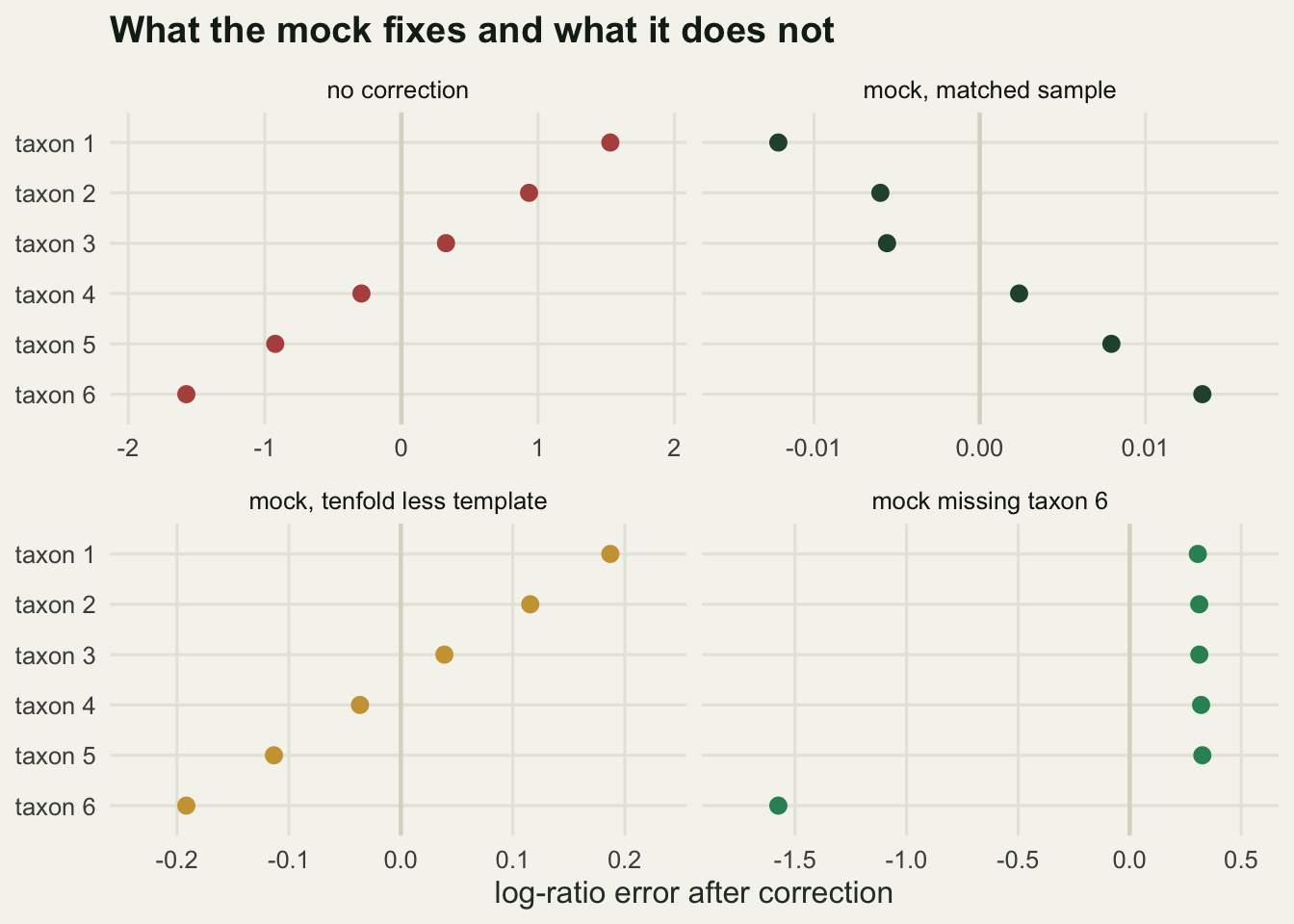

Figure 3: Per-taxon log-ratio error under four correction scenarios. Panels have independent horizontal scales because the uncorrected errors are two orders of magnitude larger than the corrected ones.

What the correction costs

A correction estimated from data adds noise. The mock is sequenced once per run like anything else, so the offset carries its own sampling error, and subtracting it moves that error into every sample. The block below tracks the log-ratio of the first taxon to the sixth across replicate runs, uncorrected and corrected, and compares both against the floor set by multinomial sampling at the sequencer.

mock_lr <- apply(mock_obs, 2, function(p) clr_of(p)[1] - clr_of(p)[6])
samp_lr <- samp_clr[1, ] - samp_clr[6, ]
corr_lr <- samp_lr - mock_lr
truth_lr <- log(p_field[1] / p_field[6])
p_final <- rowMeans(replicate(40, amplify_seq(p_field, load_std)))
ceiling_se <- sqrt(1 / (depth_reads * p_final[1]) + 1 / (depth_reads * p_final[6]))
print(round(c(sd_uncorrected = sd(samp_lr), sd_corrected = sd(corr_lr),
              multinomial_floor = ceiling_se,
              bias_uncorrected = mean(samp_lr) - truth_lr,
              fold_bias_uncorrected = exp(mean(samp_lr) - truth_lr),
              bias_corrected = mean(corr_lr) - truth_lr), 4))

       sd_uncorrected          sd_corrected     multinomial_floor 
               0.0379                0.0518                0.0375 
     bias_uncorrected fold_bias_uncorrected        bias_corrected 
               3.1046               22.2997               -0.0256 

print(round(c(rmse_uncorrected = sqrt(mean((samp_lr - truth_lr)^2)),
              rmse_corrected = sqrt(mean((corr_lr - truth_lr)^2)),
              rmse_gain = sqrt(mean((samp_lr - truth_lr)^2)) /
                          sqrt(mean((corr_lr - truth_lr)^2)),
              sd_cost = sd(corr_lr) / sd(samp_lr)), 3))

rmse_uncorrected   rmse_corrected        rmse_gain          sd_cost 
           3.105            0.058           53.851            1.366 

depth_break <- (1 / p_final[1] + 1 / p_final[6]) / resid_tab["tenfold_less", "corrected"]^2
print(round(c(depth_where_noise_matches_residual = depth_break)))

depth_where_noise_matches_residual 
                              4197 

The uncorrected log-ratio has a standard deviation of 0.0379 across runs, and the multinomial floor at 50000 reads is 0.0375. Those are almost the same number, which says the run-to-run variability of an uncorrected metabarcoding log-ratio is essentially all sequencing noise: the PCR contributes bias, not scatter. Correcting raises the standard deviation to 0.0518, a cost factor of 1.366, because the mock’s own sampling error is now in the answer.

Against that cost sits a bias of 3.1046 log-ratio units, a 22.2997-fold error, reduced to -0.0256. The root mean square error falls from 3.105 to 0.058, a gain of 53.851. The correction is worth its variance many times over, and the reason is simply that the bias is enormous and the noise is not.

That also settles the read-depth question, in the opposite direction to the one this section was set up to ask. Sequencing noise is not the limiting factor here; it is the smallest term in the run. Sequencing deeper than 50000 reads buys nothing, because the residual after correction for a sample with a tenfold template mismatch is 0.1295, more than three times the noise floor. The last line solves for the depth at which the two would be equal and gets 4197 reads. Below roughly four thousand reads for this composition, extra sequencing helps; above it, extra sequencing is decoration.

Ranking the four error sources

Four things stand between the sample and the read table, and they can be put on one scale: the root mean square distortion they impose on the centred log-ratios of a six-taxon composition. Extraction efficiency and marker copy number act together as one fixed multiplicative factor per taxon, and the spread used here is stipulated rather than measured, a log-scale standard deviation of 0.7, which is a modest assumption next to the range of ribosomal copy numbers across eukaryotes.

set.seed(20260820)
extract_sd <- 0.7
extract_fac <- exp(rnorm(n_taxa, 0, extract_sd))
extract_err <- clr_of(extract_fac)
seq_noise <- apply(replicate(n_rep_mock, {
  reads <- as.numeric(rmultinom(1, depth_reads, p_final))
  clr_of(reads / sum(reads)) - clr_of(p_final)
}), 2, function(z) sqrt(mean(z^2)))
budget <- c(`extraction and copy number` = sqrt(mean(extract_err^2)),
            `amplification efficiency` = sqrt(mean(bias_hat^2)),
            `plateau transfer error` = unname(resid_tab["tenfold_less", "corrected"]),
            `sequencing multinomial` = mean(seq_noise))
print(round(c(stipulated_extraction_log_sd = extract_sd), 2))

stipulated_extraction_log_sd 
                         0.7 

print(round(budget, 4))

extraction and copy number   amplification efficiency 
                    0.9645                     1.0685 
    plateau transfer error     sequencing multinomial 
                    0.1295                     0.0171 

print(round(budget / budget["sequencing multinomial"], 1))

extraction and copy number   amplification efficiency 
                      56.2                       62.3 
    plateau transfer error     sequencing multinomial 
                       7.5                        1.0 

Amplification efficiency is the largest at 1.0685, extraction and copy number next at 0.9645, the non-transferable part of the plateau effect at 0.1295 and sequencing noise last at 0.0171. On a common scale that is 62.3, 56.2, 7.5 and 1.

The ranking argues for a specific order of effort. The two largest terms are both fixed multiplicative factors per taxon, and a mock community removes both at once, provided the mock enters the workflow at the extraction step rather than as pooled DNA: a mock made of purified genomic DNA corrects the second-largest term only. The third term is the one a mock cannot carry, and the lever on it is matching template input between mock and samples, not more replicates. The fourth term is small enough that read depth should be the last thing on the budget. A study that spends its money on deeper sequencing and skips the mock has optimised the term that contributed one unit while ignoring the one that contributed sixty-two.

bud_dat <- data.frame(source = factor(names(budget), rev(names(budget))),
                      rms = as.numeric(budget))
p_bud <- ggplot(bud_dat, aes(rms, source)) +
  geom_segment(aes(x = 0.012, xend = rms, yend = source), colour = te_pal$sage,
               linewidth = 1.8) +
  geom_point(size = 4.2, colour = te_pal$forest) +
  geom_text(aes(label = sprintf("%.3f", rms)), hjust = -0.4, vjust = -0.7,
            size = 3.5, colour = te_pal$ink) +
  scale_x_log10(limits = c(0.012, 5)) +
  labs(title = "Where a metabarcoding run loses its quantities",
       x = "RMS log-ratio distortion", y = NULL) +
  theme_te()
p_bud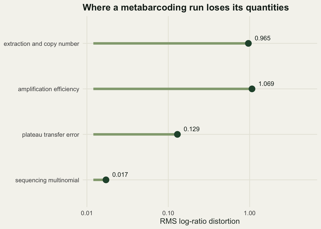

Figure 4: Root mean square log-ratio distortion from four sources in a six-taxon metabarcoding run, on a logarithmic scale. Amplification and extraction dominate; sequencing noise is two orders of magnitude smaller.

The assumption underneath all of it

Every measurement above treats the per-cycle efficiency as a property of the taxon. It is not. Amplification efficiency is a property of the interaction between a primer pair and a specific template sequence, and the thing that sets it is the number and position of mismatches in the primer binding sites. Two individuals of the same species with different haplotypes at those sites can amplify at measurably different rates, and within a species the variation across a range can be large.

That breaks the calibration in a way no amount of care in the laboratory repairs. A mock community is built from cultured strains, voucher tissue or reference extractions, so it carries one haplotype per taxon, or a few, while the field samples carry whatever the population carries. The offset estimated from the mock is the offset for the mock’s haplotypes, and the difference between that and the offset for the sample’s haplotypes is invisible from the run: no internal contrast separates it from real abundance variation.

A mock community, then, calibrates the protocol against itself. It measures how this primer pair, this polymerase and this cycling profile treat these particular templates, and it removes that. The residual is a haplotype-level bias that is unmeasurable without independent quantification of the same samples, by digital PCR of a few target taxa or by a second marker with different binding sites. The honest reporting is to say the correction was applied, to say what the mock contained, and not to claim the corrected proportions are unbiased. They are less biased by a factor this post can measure and by an amount it cannot.

Where to go next

The next post in this cluster deals with the other way a read table acquires taxa that were never in the sample: contamination, index hopping and the low-abundance reads that survive every filter. It interacts with everything measured here, because an efficiently amplifying contaminant at trace concentration can outrun a genuine prey item at real concentration. The cluster then closes with a set of diagnostics that check a finished metabarcoding analysis against the assumptions the three earlier posts made.

References

Deagle BE, Thomas AC, Shaffer AK, Trites AW, Jarman SN 2013 Molecular Ecology Resources 13(4):620-633 (10.1111/1755-0998.12103)

McLaren MR, Willis AD, Callahan BJ 2019 eLife 8:e46923 (10.7554/eLife.46923)

Nichols RV, Vollmers C, Newsom LA, Wang Y, Heintzman PD, Leighton M, Green RE, Shapiro B 2018 Molecular Ecology Resources 18(5):927-939 (10.1111/1755-0998.12895)

Pinol J, Mir G, Gomez-Polo P, Agusti N 2015 Molecular Ecology Resources 15(4):819-830 (10.1111/1755-0998.12355)

Krehenwinkel H, Wolf M, Lim JY, Rominger AJ, Simison WB, Gillespie RG 2017 Scientific Reports 7:17668 (10.1038/s41598-017-17333-x)

Gloor GB, Macklaim JM, Pawlowsky-Glahn V, Egozcue JJ 2017 Frontiers in Microbiology 8:2224 (10.3389/fmicb.2017.02224)

Related tutorials

• Metabarcoding reads as compositional data
• Contamination filtering in metabarcoding
• Checking a metabarcoding analysis
• Compositional analysis and the zero problem