library(ggplot2)
library(patchwork)

te_paper  <- "#f5f4ee"
te_ink    <- "#16241d"
te_body   <- "#2c3a31"
te_forest <- "#275139"
te_rust   <- "#b5534e"
te_gold   <- "#c9b458"
te_line   <- "#dad9ca"

theme_datasheet <- function() {
  theme_minimal(base_size = 12) +
    theme(plot.background  = element_rect(fill = te_paper, colour = NA),
          panel.background = element_rect(fill = te_paper, colour = NA),
          panel.grid.major = element_line(colour = te_line, linewidth = 0.3),
          panel.grid.minor = element_blank(),
          text             = element_text(colour = te_body),
          plot.title       = element_text(colour = te_ink, face = "bold"),
          plot.subtitle    = element_text(colour = te_body),
          axis.text        = element_text(colour = te_body))
}Dirichlet-multinomial models for read counts
R
metabarcoding
overdispersion
simulation
diet analysis
ecology tutorial
Why a multinomial interval for a metabarcoding diet share is too narrow, and how the Dirichlet-multinomial in R turns deep libraries into a few hundred reads.
A colony of brown long-eared bats roosts in a church loft, and eight fresh faecal pellets are collected from the floor under the roost in a single morning. Each pellet is extracted, amplified with an arthropod marker and sequenced to twenty thousand reads, and the reads are assigned to six prey orders. The question is simple: what share of the colony diet is made up of caddisflies? The pooled table holds a hundred and sixty thousand reads, and the obvious interval treats them as a hundred and sixty thousand independent draws from one set of prey proportions. That interval is very narrow, and it is wrong.
This post writes down the likelihood that the obvious interval assumes, the multinomial, and the one that should replace it, the Dirichlet-multinomial. It sits inside a cluster that has already taken the read table apart. Metabarcoding reads as compositional data generates its libraries with a multinomial draw and establishes that a read table carries ratios only. PCR bias and amplification efficiency uses the multinomial as the noise floor of a single run and finds that, for one template sequenced again and again, run-to-run scatter in a log-ratio is almost all sequencing noise. Here the template changes from pellet to pellet, and that is the case in which the multinomial floor stops being the right yardstick.
The closest neighbour is Check three of Checking a metabarcoding analysis. That check puts a design effect of one plus the number of replicates minus one times an intraclass correlation on the replicate axis, and finds that 216 rows of extractions and PCRs from 24 animals carry the information of about 39 independent observations. The same arithmetic applies one level lower, inside a single library, with reads in place of PCR replicates. It is less intuitive there, because a read looks like a physical, countable, independent thing in a way a PCR replicate does not, and because the number of reads per library is in the tens of thousands rather than single figures.
Two likelihoods for one read table
The multinomial says that every pellet has the same prey proportions and that each read is an independent draw from them. The Dirichlet-multinomial, set out by Mosimann 1962 as the compound multinomial, first draws a pellet’s own proportions from a Dirichlet distribution and then draws the reads from those. The parameterisation used throughout is the one with a mean vector and one overdispersion parameter. The Dirichlet parameters are the colony mean proportions times a concentration, and the concentration is one minus theta, divided by theta. Theta is the correlation between the prey identities of two reads from the same library, and with a concentration of infinity it is zero and the model is the multinomial again.
With that parameterisation the variance of a read count for one prey order in a library of n reads is the multinomial variance multiplied by one plus n minus one times theta. The multiplier is the same design effect as in Check three, and dividing the library size by it gives the effective depth, the number of independent reads that would carry the same information about the colony proportion. As n grows the effective depth does not grow without limit; it approaches one over theta.
The design constants are fixed here and not touched afterwards: six prey orders with colony shares from forty per cent down to three per cent, caddisflies at ten per cent, eight pellets, twenty thousand reads each, and a theta of three thousandths.
prey      <- c("Lepidoptera", "Diptera", "Coleoptera", "Trichoptera",
               "Neuroptera", "Araneae")
pi_true   <- c(0.40, 0.25, 0.15, 0.10, 0.07, 0.03)   # colony diet shares
focal     <- 4                                        # Trichoptera
theta_set <- 0.003                                    # read to read correlation
conc_set  <- (1 - theta_set) / theta_set              # Dirichlet concentration
alpha_set <- pi_true * conc_set                       # Dirichlet parameters
n_pellet  <- 8
depth_set <- 20000
z_crit    <- qnorm(0.975)
n_eff_of  <- function(n, theta) n / (1 + (n - 1) * theta)

# one dataset: pellet proportions from the Dirichlet, reads from the multinomial
sim_dm <- function(J, n, alpha) {
  K <- length(alpha)
  props <- matrix(rgamma(J * K, rep(alpha, each = J)), nrow = J)
  props <- props / rowSums(props)
  reads <- t(apply(props, 1, function(p) rmultinom(1, n, p)))
  list(props = props, reads = reads)
}
The Dirichlet-multinomial log-likelihood is a few lines of lgamma, and its gradient is the same lines with digamma. Both are written on the log scale of the Dirichlet parameters so the optimiser is unconstrained. The multinomial coefficient does not involve the parameters and is left out of the fitting function; the check below puts it back.
dm_loglik <- function(eta, reads) {
  a <- exp(eta); a_sum <- sum(a); lib <- rowSums(reads)
  sum(lgamma(a_sum) - lgamma(lib + a_sum)) +
    sum(lgamma(sweep(reads, 2, a, "+"))) - nrow(reads) * sum(lgamma(a))
}
dm_grad <- function(eta, reads) {
  a <- exp(eta); a_sum <- sum(a); lib <- rowSums(reads)
  a * (sum(digamma(a_sum) - digamma(lib + a_sum)) +
       colSums(digamma(sweep(reads, 2, a, "+"))) - nrow(reads) * digamma(a))
}

# two prey orders: the Dirichlet-multinomial is the beta-binomial, so the
# closed form can be checked against numerical integration over the beta
chk_a <- c(2.5, 7.5); chk_x <- c(13, 27); chk_n <- sum(chk_x)
ll_closed <- dm_loglik(log(chk_a), matrix(chk_x, nrow = 1)) +
  lgamma(chk_n + 1) - sum(lgamma(chk_x + 1))
ll_numeric <- log(integrate(function(p) dbinom(chk_x[1], chk_n, p) *
                              dbeta(p, chk_a[1], chk_a[2]), 0, 1)$value)
ll_gap <- abs(ll_closed - ll_numeric)

# the variance of a read count against the design effect formula
set.seed(24081)
var_draws <- sim_dm(20000, depth_set, alpha_set)$reads[, focal]
var_ratio <- var(var_draws) / (depth_set * pi_true[focal] * (1 - pi_true[focal]))
deff_set  <- 1 + (depth_set - 1) * theta_set
The closed form and the numerical integral agree to 9.1e-14 on the log scale. Across twenty thousand simulated libraries the variance of the caddisfly read count is 60.6 times the multinomial variance, against a design effect of 61.0 from the formula. A library of 20000 reads at this theta has an effective depth of 328, and the ceiling for an infinitely deep library is 333.
Fitting both models to eight pellets
The multinomial fit is the pooled proportion, and its Wald interval uses the total read count. The Dirichlet-multinomial fit is maximised with nlminb and the analytic gradient, from a moment starting value, and its interval for a prey share comes from the inverse of the observed information on the log parameter scale, carried to the proportion scale by the delta method. The concentration can run off to infinity when the pellets happen to agree more closely than the multinomial expects; the fitted theta is then zero, the Dirichlet-multinomial has become the multinomial, and the function says so and returns the multinomial answer.
fit_dm <- function(reads) {
  p_pool <- colSums(reads) / sum(reads)
  lib <- mean(rowSums(reads))
  p_row <- reads / rowSums(reads)
  th0 <- (mean(apply(p_row, 2, var) / (p_pool * (1 - p_pool))) - 1 / lib)
  th0 <- min(0.5, max(1e-4, th0))
  # nlminb minimises, so both functions change sign; optim's BFGS was tried
  # first and its line search jumped to concentrations of 1e20 and more, where
  # the lgamma differences in dm_loglik lose all precision and return a false maximum
  opt <- nlminb(log(p_pool * (1 - th0) / th0), function(e) -dm_loglik(e, reads),
                function(e) -dm_grad(e, reads))
  a <- exp(opt$par); theta_hat <- 1 / (1 + sum(a))
  if (theta_hat < 1e-6) {
    return(list(p = p_pool, se = sqrt(p_pool * (1 - p_pool) / sum(reads)),
                theta = 0, boundary = TRUE, se_logit_theta = NA, loglik = NA))
  }
  vcov_eta <- solve(-optimHess(opt$par, dm_loglik, dm_grad, reads = reads))
  p_hat <- a / sum(a)
  jac <- diag(p_hat) - outer(p_hat, p_hat)
  # logit(theta) is minus the log of the concentration, whose gradient is p_hat
  list(p = p_hat, se = sqrt(diag(jac %*% vcov_eta %*% jac)), theta = theta_hat,
       boundary = FALSE, se_logit_theta = sqrt(drop(p_hat %*% vcov_eta %*% p_hat)),
       loglik = -opt$objective)
}
fit_mult <- function(reads) {
  p_pool <- colSums(reads) / sum(reads)
  list(p = p_pool, se = sqrt(p_pool * (1 - p_pool) / sum(reads)))
}

set.seed(24082)
ex <- sim_dm(n_pellet, depth_set, alpha_set)
ex_m <- fit_mult(ex$reads); ex_d <- fit_dm(ex$reads)
ex_share <- ex$reads[, focal] / depth_set
ex_ci_m <- ex_m$p[focal] + c(-1, 1) * z_crit * ex_m$se[focal]
ex_ci_d <- ex_d$p[focal] + c(-1, 1) * z_crit * ex_d$se[focal]
ex_theta_ci <- plogis(qlogis(ex_d$theta) + c(-1, 1) * z_crit * ex_d$se_logit_theta)
ex_neff_ci <- n_eff_of(depth_set, rev(ex_theta_ci))
ex_ll_mult <- sum(ex$reads * log(rep(ex_m$p, each = n_pellet)))
ex_lr <- 2 * (ex_d$loglik + sum(lgamma(rowSums(ex$reads) + 1)) - sum(lgamma(ex$reads + 1)) -
              (ex_ll_mult + sum(lgamma(rowSums(ex$reads) + 1)) - sum(lgamma(ex$reads + 1))))
ex_ratio_se <- ex_d$se[focal] / ex_m$se[focal]
lr_crit <- qchisq(0.90, df = 1)   # 5 per cent point of the 50:50 boundary mixture
In this dataset the eight pellets give caddisfly shares from 0.081 to 0.127. The multinomial interval for the colony share is 0.101 to 0.103, which excludes 7 of the eight pellets it was computed from. The Dirichlet-multinomial interval is 0.092 to 0.112, 6.7 times wider. The fitted theta is 0.0022 with a Wald interval from 0.0014 to 0.0034, so each twenty thousand read library is worth between 289 and 691 independent reads. The likelihood ratio statistic for theta against zero is 1619. Because a theta of zero sits on the edge of the parameter space, its null distribution is half a chi-square with one degree of freedom and half a point mass at zero; the five per cent critical value of that mixture is 2.71, and this statistic is far beyond it.
pel <- data.frame(label = sprintf("pellet %d", seq_len(n_pellet)), est = ex_share,
                  lo = ex_share - z_crit * sqrt(ex_share * (1 - ex_share) / depth_set),
                  hi = ex_share + z_crit * sqrt(ex_share * (1 - ex_share) / depth_set),
                  kind = "one library, multinomial")
pooled <- data.frame(label = c("pooled, multinomial", "pooled, Dirichlet-multinomial"),
                     est = c(ex_m$p[focal], ex_d$p[focal]),
                     lo = c(ex_ci_m[1], ex_ci_d[1]), hi = c(ex_ci_m[2], ex_ci_d[2]),
                     kind = c("colony, multinomial", "colony, Dirichlet-multinomial"))
pel_all <- rbind(pel, pooled)
pel_all$label <- factor(pel_all$label, levels = rev(pel_all$label))
pel_all$kind <- factor(pel_all$kind, levels = c("one library, multinomial",
                       "colony, multinomial", "colony, Dirichlet-multinomial"))
ggplot(pel_all, aes(est, label, colour = kind)) +
  geom_vline(xintercept = pi_true[focal], colour = te_body, linetype = "dashed",
             linewidth = 0.5) +
  geom_errorbar(aes(xmin = lo, xmax = hi), orientation = "y", width = 0.35,
                linewidth = 0.7) +
  geom_point(size = 2.4) +
  scale_colour_manual(values = c(te_gold, te_rust, te_forest), name = NULL) +
  guides(colour = guide_legend(nrow = 2)) +
  labs(x = "caddisfly share of reads", y = NULL,
       title = "Eight pellets, two answers for the colony",
       subtitle = "dashed line: the colony share used to simulate") +
  theme_datasheet() + theme(legend.position = "bottom")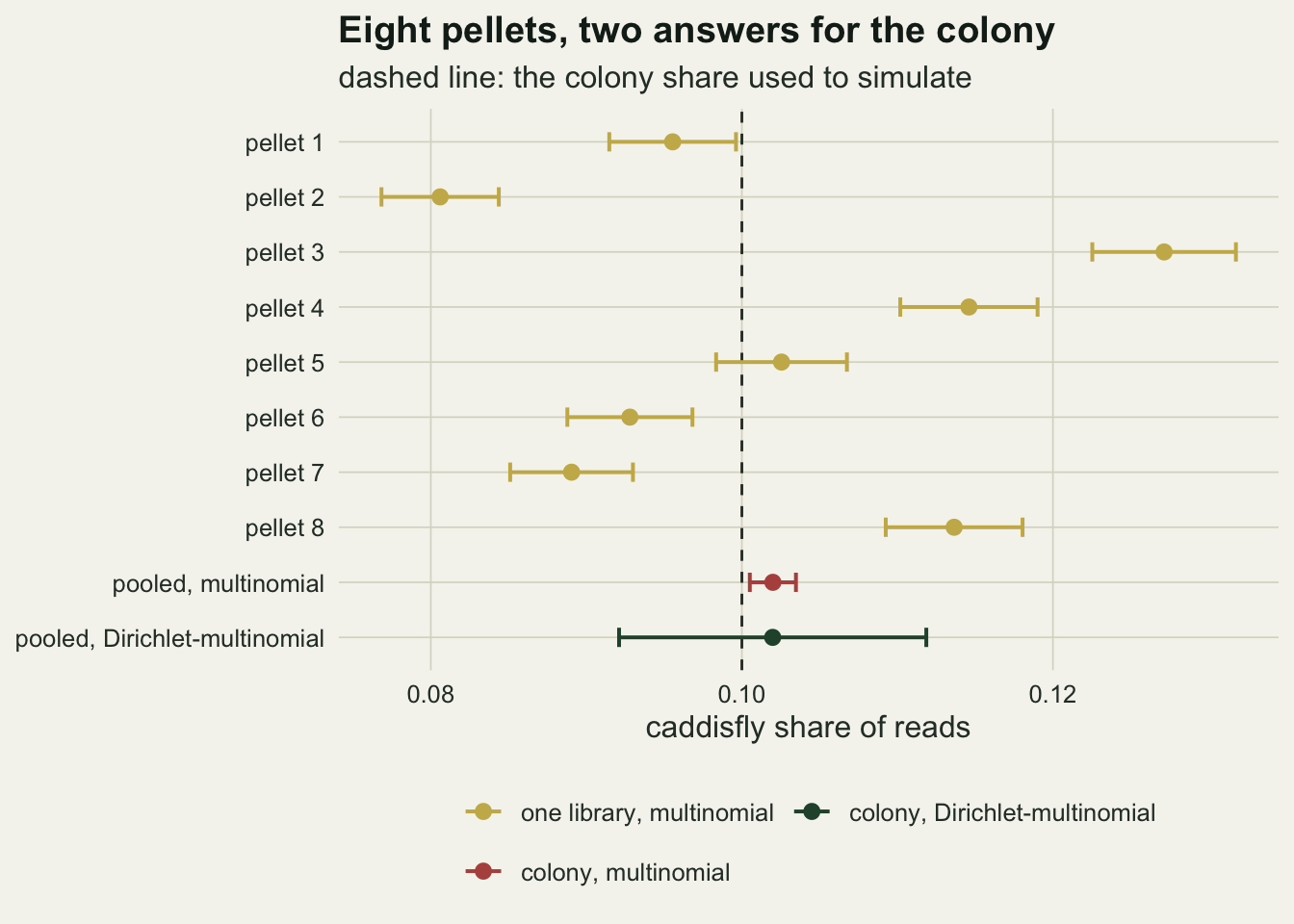
Coverage against sequencing depth
One dataset shows the shape of the problem; coverage needs many. For each of six library sizes, a thousand datasets of eight pellets are drawn and both models fitted. Three coverages are plotted. Two are for the colony share, the target a diet study reports. The third is the multinomial interval from one library for that pellet’s own proportion, the Dirichlet draw that generated its reads, which is the quantity the multinomial is actually a model of.
n_rep <- 1000                     # datasets per setting, fixed before running
depth_grid <- c(500, 1000, 2000, 5000, 20000, 80000)
run_setting <- function(J, n) {
  out <- vapply(seq_len(n_rep), function(i) {
    s <- sim_dm(J, n, alpha_set)
    m <- fit_mult(s$reads); d <- fit_dm(s$reads)
    own <- s$reads[, focal] / n
    own_se <- sqrt(own * (1 - own) / n)
    # the design effect formula for the standard error, with the fitted and
    # with the true theta, and the fitted interval with a t quantile on J - 1 df
    se_form <- function(th) sqrt(d$p[focal] * (1 - d$p[focal]) * (1 + (n - 1) * th) / (J * n))
    c(cov_mult = abs(m$p[focal] - pi_true[focal]) <= z_crit * m$se[focal],
      cov_dm   = abs(d$p[focal] - pi_true[focal]) <= z_crit * d$se[focal],
      cov_dm_form = abs(d$p[focal] - pi_true[focal]) <= z_crit * se_form(d$theta),
      cov_dm_true = abs(d$p[focal] - pi_true[focal]) <= z_crit * se_form(theta_set),
      cov_dm_t = abs(d$p[focal] - pi_true[focal]) <= qt(0.975, J - 1) * d$se[focal],
      cov_own  = mean(abs(own - s$props[, focal]) <= z_crit * own_se),
      cov_mean = abs(m$p[focal] - mean(s$props[, focal])) <= z_crit * m$se[focal],
      wid_mult = 2 * z_crit * m$se[focal], wid_dm = 2 * z_crit * d$se[focal],
      theta = d$theta, boundary = d$boundary,
      pool_gap = max(abs(d$p - m$p)))
  }, numeric(12))
  data.frame(J = J, n = n, t(out))
}
set.seed(24083)
sims <- do.call(rbind, lapply(depth_grid, function(n) run_setting(n_pellet, n)))
cov_tab <- aggregate(cbind(cov_mult, cov_dm, cov_dm_form, cov_dm_true, cov_dm_t, cov_own, cov_mean,
                           wid_mult, wid_dm, boundary) ~ n, data = sims, FUN = mean)
# cov_own averages eight intervals per dataset, so its Monte Carlo error comes
# from the spread of the per-dataset rates, not from a binomial count of datasets
mcse_own <- aggregate(cov_own ~ n, data = sims, FUN = function(v) sd(v) / sqrt(length(v)))
at_n <- function(col, n) cov_tab[[col]][cov_tab$n == n]
mcse_of <- function(p) sqrt(p * (1 - p) / n_rep)
max_pool_gap <- max(sims$pool_gap)
At 20000 reads per pellet the multinomial interval covers the colony caddisfly share in 21.2 per cent of datasets. The Dirichlet-multinomial interval covers it in 92.4 per cent, with a Monte Carlo standard error of 0.8 percentage points. The single-library multinomial interval covers its own pellet’s proportion 95.1 per cent of the time, and the pooled multinomial interval covers the average proportion of the eight pellets actually collected in 94.3 per cent of datasets: it describes those pellets, not the colony. The multinomial is not a bad model of reads; it is a good model of the wrong target.
Across the depth grid the multinomial coverage for the colony share falls from 77.3 per cent at 500 reads to 10.4 per cent at 80000. The Dirichlet-multinomial coverage runs between 91.8 and 92.7 per cent over the same range. It is flat, but it sits below ninety five per cent at every depth: the highest point plus two Monte Carlo standard errors reaches only 94.3 per cent. The design effect formula gives a second standard error around the same point estimates. With the fitted theta in it, coverage runs between 91.9 and 92.9 per cent, much as the fitted interval does; with the true theta it runs between 94.8 and 95.6 per cent, so the shortfall comes from estimating theta from eight pellets. The two models give nearly the same point estimate: the largest difference between the fitted and the pooled proportion of any prey order, over all 6000 fits, is 0.0036. Only the width differs.
cov_long <- data.frame(
  n = rep(cov_tab$n, 3),
  coverage = c(cov_tab$cov_own, cov_tab$cov_dm, cov_tab$cov_mult),
  interval = factor(rep(c("multinomial, own pellet proportion",
                          "Dirichlet-multinomial, colony share",
                          "multinomial, colony share"), each = nrow(cov_tab)),
                    levels = c("multinomial, own pellet proportion",
                               "Dirichlet-multinomial, colony share",
                               "multinomial, colony share")))
cov_long$mcse <- mcse_of(cov_long$coverage)
cov_long$mcse[cov_long$interval == "multinomial, own pellet proportion"] <- mcse_own$cov_own
ggplot(cov_long, aes(n, coverage, colour = interval)) +
  geom_hline(yintercept = 0.95, colour = te_body, linetype = "dashed", linewidth = 0.5) +
  geom_errorbar(aes(ymin = coverage - 2 * mcse, ymax = coverage + 2 * mcse),
                width = 0.06, linewidth = 0.4) +
  geom_line(linewidth = 0.9) + geom_point(size = 2.2) +
  scale_x_log10(breaks = depth_grid, labels = format(depth_grid, big.mark = ",",
                                                     scientific = FALSE, trim = TRUE)) +
  scale_colour_manual(values = c(te_gold, te_forest, te_rust), name = NULL) +
  scale_y_continuous(limits = c(0, 1)) +
  guides(colour = guide_legend(nrow = 3)) +
  labs(x = "reads per pellet (log scale)", y = "coverage",
       title = "More reads make the wrong interval worse",
       subtitle = "dashed line: nominal 95 per cent") +
  theme_datasheet() + theme(legend.position = "bottom")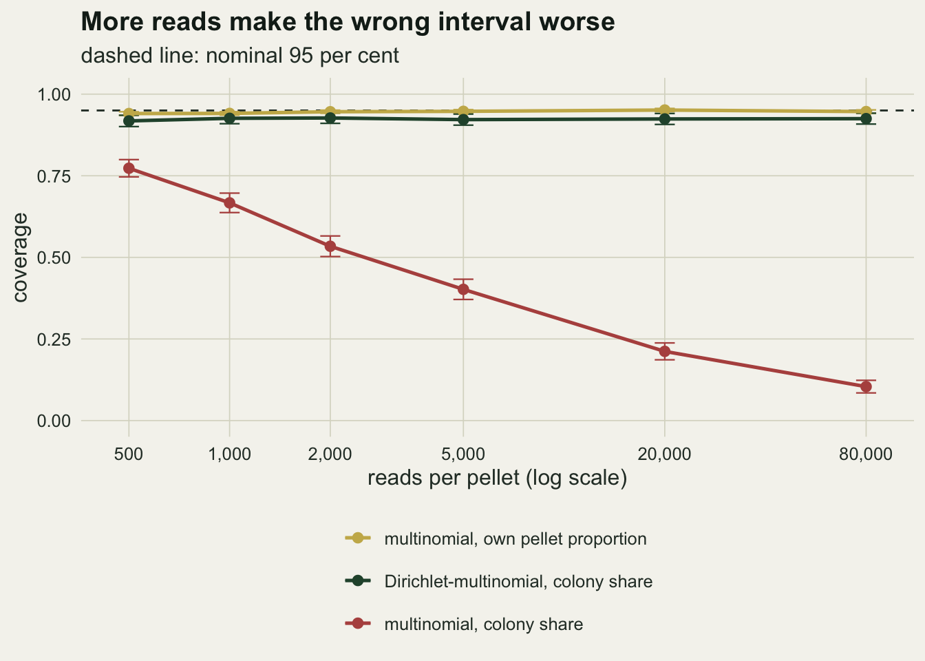
The effective depth is a few hundred reads
Each fit returns a theta, and each theta converts to an effective depth. The truth is a curve that bends over towards one over theta; what eight pellets estimate is scattered about it, and the median of the estimates sits above it at every depth.
sims$neff <- n_eff_of(sims$n, sims$theta)
neff_tab <- do.call(rbind, lapply(depth_grid, function(n) {
  v <- sims$neff[sims$n == n]
  data.frame(n = n, med = median(v), lo = unname(quantile(v, 0.1)),
             hi = unname(quantile(v, 0.9)), truth = n_eff_of(n, theta_set))
}))
theta_main <- sims$theta[sims$n == depth_set]
theta_med <- median(theta_main); theta_mean <- mean(theta_main)
nb_main <- neff_tab[neff_tab$n == depth_set, ]
n_boundary <- sum(sims$boundary); boundary_500 <- at_n("boundary", 500)
share_of_nominal <- nb_main$truth / depth_set
At 20000 reads the true effective depth is 328, which is 1.6 per cent of the reads sequenced. The median estimate across a thousand datasets is 386, and the middle eighty per cent of estimates runs from 286 to 530. The median estimate sits above the truth because theta is estimated low: its median is 0.00254 and its mean 0.00258 against the 0.003 used to simulate. A maximum likelihood variance component from eight groups is biased towards zero, and here that bias shows up as an effective depth that is too generous, which is the reason the interval is a little too narrow: with the true theta the coverage of the previous section returns to nominal.
Theta hit its boundary at zero in 4 of the 6000 fits, a rate of 0.4 per cent among the fits at 500 reads, and never at a depth above 500 reads. At shallow depth the multinomial noise is large enough that eight pellets can look homogeneous by chance.
curve_n <- 10^seq(log10(300), log10(1e5), length.out = 200)
curve_df <- data.frame(n = curve_n, neff = n_eff_of(curve_n, theta_set))
ggplot(neff_tab, aes(n, med)) +
  geom_line(data = curve_df, aes(n, n), colour = te_body, linetype = "dotted",
            linewidth = 0.6) +
  geom_hline(yintercept = 1 / theta_set, colour = te_body, linetype = "dashed",
             linewidth = 0.5) +
  geom_line(data = curve_df, aes(n, neff), colour = te_forest, linewidth = 1) +
  geom_errorbar(aes(ymin = lo, ymax = hi), width = 0.06, colour = te_rust,
                linewidth = 0.6) +
  geom_point(colour = te_rust, size = 2.4) +
  scale_x_log10(breaks = depth_grid, labels = format(depth_grid, big.mark = ",",
                                                     scientific = FALSE, trim = TRUE)) +
  scale_y_log10(breaks = c(100, 200, 500, 1000, 5000, 20000, 1e5),
                labels = format(c(100, 200, 500, 1000, 5000, 20000, 1e5),
                                big.mark = ",", scientific = FALSE, trim = TRUE)) +
  coord_cartesian(ylim = c(100, 1e5)) +
  labs(x = "reads per pellet (log scale)", y = "effective reads (log scale)",
       title = "Twenty thousand reads, a few hundred worth of information",
       subtitle = "green line: formula, points: estimates\ndotted: independent reads, dashed: one over theta") +
  theme_datasheet()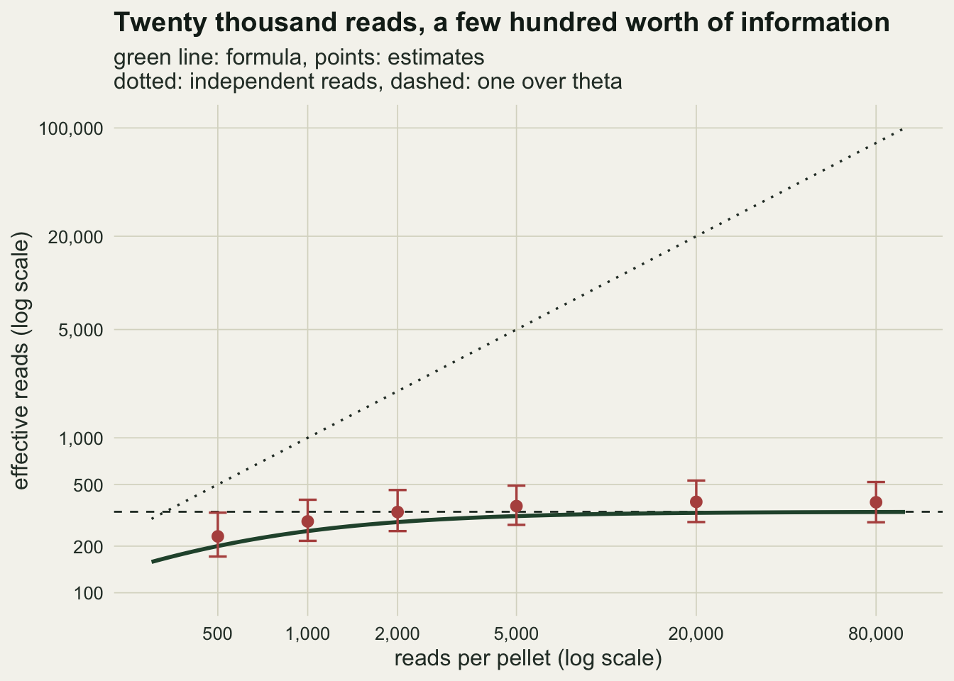
Pellets buy precision, reads do not
The variance of the pooled caddisfly share under the Dirichlet-multinomial is the multinomial variance for one library, times the design effect, divided by the number of pellets. As the library grows that tends to the share times one minus the share, times theta, over the number of pellets: a floor set by the pellets, which no sequencing depth can lower. Pellets are the other direction to spend effort, so the same thousand-dataset run is repeated at twenty thousand reads for four, sixteen and thirty two pellets.
j_grid <- c(4, 8, 16, 32)
set.seed(24084)
sims_j <- rbind(sims[sims$n == depth_set, names(sims) != "neff"],
                do.call(rbind, lapply(setdiff(j_grid, n_pellet),
                                      function(J) run_setting(J, depth_set))))
j_tab <- aggregate(cbind(cov_mult, cov_dm, cov_dm_true, cov_dm_t, wid_dm, boundary) ~ J,
                   data = sims_j, FUN = mean)
width_theory <- function(n, J, theta) 2 * z_crit * sqrt(pi_true[focal] * (1 - pi_true[focal]) *
                                                         (1 + (n - 1) * theta) / (J * n))
floor_8  <- 2 * z_crit * sqrt(pi_true[focal] * (1 - pi_true[focal]) * theta_set / n_pellet)
wid_8_20k <- width_theory(depth_set, n_pellet, theta_set)
wid_8_80k <- width_theory(80000, n_pellet, theta_set)
wid_32_20k <- width_theory(depth_set, 32, theta_set)
wid_16_2k <- width_theory(2000, 16, theta_set)
wid_sim_20k <- at_n("wid_dm", depth_set); wid_mult_20k <- at_n("wid_mult", depth_set)
at_j <- function(col, J) j_tab[[col]][j_tab$J == J]
With eight pellets the formula gives an interval 0.0230 wide at 20000 reads and 0.0228 wide at 80000, against a floor of 0.0228 for unlimited reads. Quadrupling the sequencing narrows the interval by 0.6 per cent. Quadrupling the pellets at the same depth takes it to 0.0115, a 50.0 per cent reduction. Sixteen pellets at 2000 reads, 20 per cent of the total reads of the eight-pellet design, give 0.0174.
Those widths use the true theta. The intervals actually computed from eight pellets at 20000 reads averaged 0.0211, narrower than the formula, which is consistent with the downward bias in theta from the previous section. The multinomial intervals in the same datasets averaged 0.0029.
The simulated Dirichlet-multinomial coverage at 20000 reads is 89.2 per cent with four pellets, 92.4 with eight, 94.2 with sixteen and 94.1 with thirty two. The multinomial coverage at the same four sizes is 19.5, 21.2, 22.4 and 19.7 per cent. With the true theta in the design effect formula the coverage is 95.2 per cent with four pellets and 95.1 with thirty two.
w_n <- 10^seq(log10(300), log10(1e5), length.out = 200)
w_lev <- sprintf("%d pellets", c(4, 8, 32))
w_df <- do.call(rbind, lapply(c(4, 8, 32), function(J)
  data.frame(n = w_n, width = width_theory(w_n, J, theta_set),
             pellets = factor(sprintf("%d pellets", J), levels = w_lev))))
w_floor <- data.frame(pellets = factor(w_lev, levels = w_lev),
  floor_w = 2 * z_crit * sqrt(pi_true[focal] * (1 - pi_true[focal]) * theta_set / c(4, 8, 32)))
w_sim <- data.frame(n = cov_tab$n, width = cov_tab$wid_dm,
                    pellets = factor(w_lev[2], levels = w_lev))
p_width <- ggplot(w_df, aes(n, width, colour = pellets)) +
  geom_hline(data = w_floor, aes(yintercept = floor_w, colour = pellets),
             linetype = "dashed", linewidth = 0.5) +
  geom_line(linewidth = 0.9) +
  geom_point(data = w_sim, shape = 21, size = 2.2, fill = te_paper, stroke = 0.8,
             show.legend = FALSE) +
  scale_x_log10(breaks = c(500, 5000, 50000),
                labels = c("500", "5,000", "50,000")) +
  scale_colour_manual(values = c(te_gold, te_forest, te_rust), name = NULL) +
  scale_y_continuous(limits = c(0, NA)) +
  labs(x = "reads per pellet (log scale)", y = "interval width",
       title = "Width of the interval",
       subtitle = "dashed: floor\ncircles: simulated, 8 pellets") +
  theme_datasheet() + theme(legend.position = "bottom")

j_long <- data.frame(J = rep(j_tab$J, 2), coverage = c(j_tab$cov_dm, j_tab$cov_mult),
  interval = factor(rep(c("Dirichlet-multinomial", "multinomial"), each = nrow(j_tab)),
                    levels = c("Dirichlet-multinomial", "multinomial")))
j_long$mcse <- mcse_of(j_long$coverage)
p_jcov <- ggplot(j_long, aes(J, coverage, colour = interval)) +
  geom_hline(yintercept = 0.95, colour = te_body, linetype = "dashed", linewidth = 0.5) +
  geom_errorbar(aes(ymin = coverage - 2 * mcse, ymax = coverage + 2 * mcse),
                width = 0.06, linewidth = 0.4) +
  geom_line(linewidth = 0.9) + geom_point(size = 2.2) +
  scale_x_log10(breaks = j_grid) +
  scale_colour_manual(values = c(te_forest, te_rust), name = NULL) +
  scale_y_continuous(limits = c(0, 1)) +
  labs(x = "pellets (log scale)", y = "coverage", title = "Coverage, 20,000 reads",
       subtitle = "dashed line: nominal\n95 per cent") +
  theme_datasheet() + theme(legend.position = "bottom")

p_width + p_jcov + plot_annotation(theme = theme_datasheet())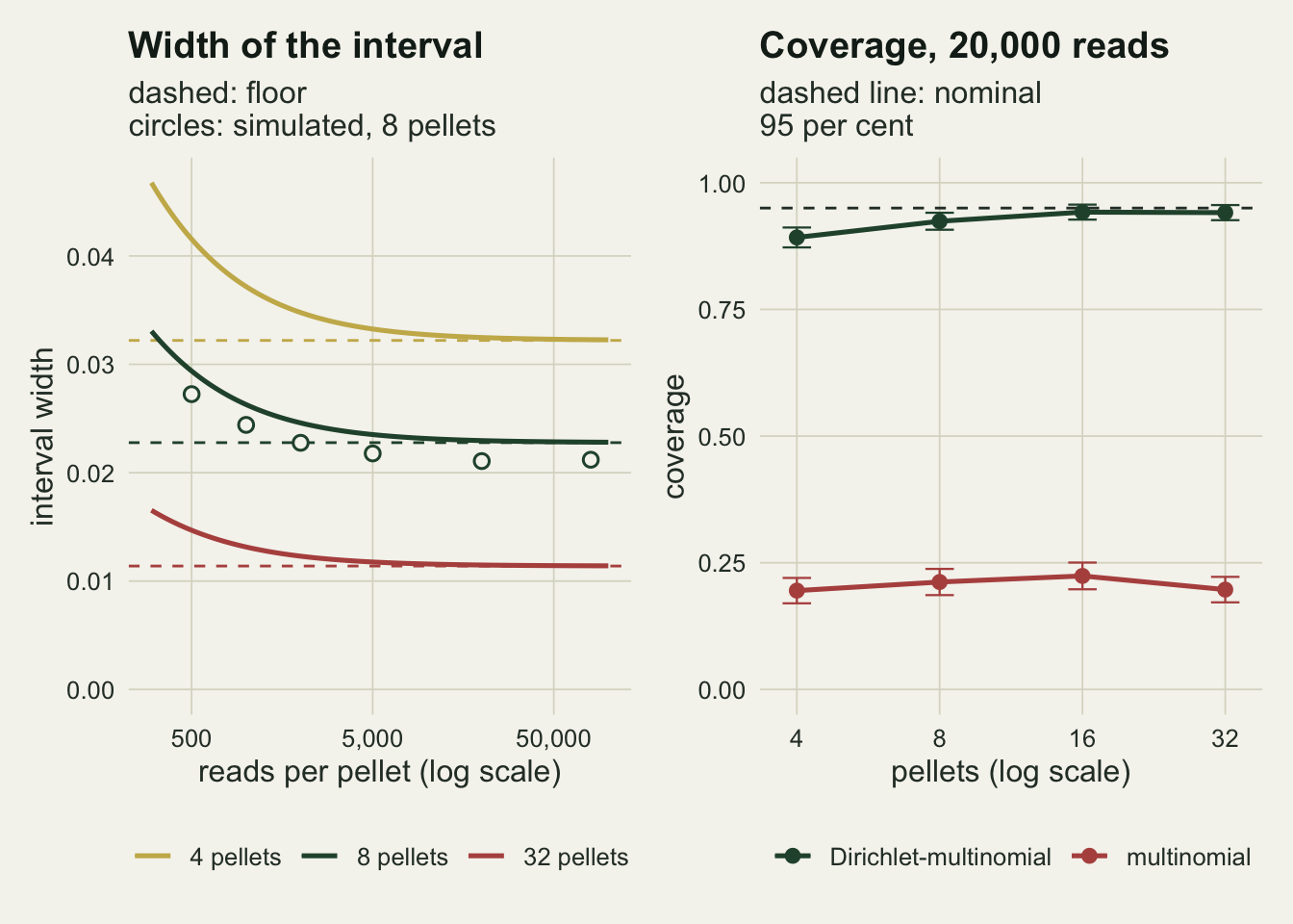
What to report
Report theta, or the concentration, with an interval, and translate it into an effective depth at the library size used. A sentence saying that each library of 20000 reads carried the information of between 289 and 691 independent reads tells a reader more about the precision of a diet share than the sequencing depth does.
State the target of every interval. An interval for a pellet’s own read share and an interval for the colony diet share are different objects, and a multinomial interval is correct for the first and far too narrow for the second. Diet papers almost always mean the second.
Report the number of independent samples, pellets here, as the sample size of any population-level proportion, and give the reads per sample as a secondary design detail. The floor on precision is set by the samples, and at the overdispersion simulated here the reads stopped mattering well below the depths common in metabarcoding.
If a likelihood is fitted, say which parameterisation of the Dirichlet-multinomial was used. The concentration, theta and the alpha vector are all in circulation, and a theta of 0.003 is a concentration of 332.3. A large concentration means little overdispersion; a large theta means a lot.
Honest limits
The Dirichlet puts one correlation on every prey order. Under it the variance of every share is inflated by the same design effect, and two prey orders can only covary negatively through closure. Real pellets can have a caddisfly share that varies a great deal between bats and a spider share that hardly varies at all, and a positive association between two prey caught in the same habitat. A logistic-normal model relaxes that, at the cost of far more parameters than eight pellets can support. The mixture of Dirichlet-multinomials that Holmes and colleagues 2012 fitted to gut microbe counts goes a different way: samples fall into several community types, each with its own Dirichlet, which suits many samples of unlike communities rather than eight pellets from one roost.
Theta here lumps together two things a study might want apart: genuine differences between bats in what they ate, and technical variation in extraction and amplification of the same meal. With one library per pellet they are not separable. Replicate extractions from one pellet, with replicate PCRs from each extract, as in Check three of the metabarcoding checks, would separate them, and the model would then need extra levels.
The interval that was measured is a Wald interval for the proportion, with its variance carried by the delta method from the information on the log parameter scale, a normal quantile and a plug-in theta. Its coverage ran below nominal at eight pellets, and the oracle run with the true theta shows that the plug-in theta is the cause. The obvious small-sample patch does not fix it cleanly: the same interval with a t quantile on the number of pellets minus one degrees of freedom covers in 98.2 per cent of datasets with four pellets and 96.9 with eight, so it trades a short interval for a long one. A profile likelihood interval for the share was not tried, and no claim is made that it repairs the coverage.
All libraries had exactly the same depth. With unequal depths the multinomial pooled estimate weights deep libraries heavily, which is wrong when pellets are the unit, while under the Dirichlet-multinomial the information in a library levels off near its effective depth, so deep libraries should count for less. The size of that difference was not measured.
The multinomial layer assumes reads are assigned to prey orders without error and that amplification is unbiased. Neither is true; PCR bias and amplification efficiency shows that bias alone can move a log-ratio by several units on the log scale. The Dirichlet-multinomial handles scatter, not bias, and a colony share estimated with a perfect interval can still be a biased estimate of what the bats ate. Harrison and colleagues 2020 found that hierarchical Dirichlet-multinomial models detected shifts in proportions between groups better than the alternatives they tried on simulated counts, and their comparison, like this one, is about relative abundance in the sequenced material, not about the biomass that went in.
References
Mosimann JE 1962 Biometrika 49(1-2):65-82 (10.1093/biomet/49.1-2.65)
Holmes I, Harris K, Quince C 2012 PLoS ONE 7(2):e30126 (10.1371/journal.pone.0030126)
Harrison JG, Calder WJ, Shastry V, Buerkle CA 2020 Molecular Ecology Resources 20(2):481-497 (10.1111/1755-0998.13128)