library(ggplot2)

te_pal <- list(forest = "#275139", green = "#2f8f63", sage = "#93a87f",
               clay = "#b5534e", gold = "#cda23f", line = "#dad9ca",
               ink = "#16241d", paper = "#f5f4ee")

theme_te <- function() {
  theme_minimal(base_size = 12) +
    theme(panel.grid.minor = element_blank(),
          panel.grid.major = element_line(colour = "#e7e6dc"),
          plot.background = element_rect(fill = "#f5f4ee", colour = NA),
          panel.background = element_rect(fill = "#f5f4ee", colour = NA),
          plot.title = element_text(face = "bold", colour = te_pal$ink),
          axis.title = element_text(colour = "#2c3a31"))
}Contamination filtering in metabarcoding
R
metabarcoding
diet analysis
model diagnostics
ecology tutorial
ggplot2
Filtering a DNA metabarcoding read table in R: cross-contamination, reagent DNA and index hopping scored against four filtering rules with a known truth.
A metabarcoding read table arrives with more sequences in it than were ever in the samples. Some of them came from the neighbouring well, some came out of a bottle of buffer, and some belong to a different library on the same flow cell. The first post of this cluster, Metabarcoding reads as compositional data, took the table as given and asked what its numbers mean; the second, PCR bias and amplification efficiency, measured what the amplification step does to them. This post is about the step in between the two and the analysis: deciding which cells of the table to set to zero.
That decision is usually made with a one-line rule. Drop anything below fifty reads. Drop anything below 0.1 per cent of the sample. Subtract the maximum seen in the negative controls. Each of these is a classifier with a tuning parameter, applied to thousands of cells, and each has a sensitivity and a specificity that nobody measures because the truth is not available in a real dataset. In a simulation it is, so the rules can be scored.
The plan is a read table with three kinds of contamination in it, each with its own statistical signature, then four filtering rules swept across their tuning parameters and scored on that table. After that, the two questions that matter more than the scores: which rule catches which source, and what filtering does to the ecological estimate. Contamination can also be modelled inside the analysis instead of removed before it, which is what False positives in eDNA surveys does with an occupancy likelihood. Here everything happens on the read table, before any model is fitted.
A run with three contaminant sources
The setting is a diet study: faecal samples on a plate, one marker, one sequencing run. Six of the wells hold extraction blanks, and every well is a library on the same flow cell. Sample DNA concentration spans two orders of magnitude, as faecal and other low-biomass material does, and it is the covariate that separates one contaminant source from another.
The three sources are built in terms of DNA mass, not reads, because that is where they differ. Cross-contamination moves a fraction of a well’s DNA into its plate neighbours, so the amount delivered is proportional to the donor’s concentration and composition, and the leak rate is patchy across the plate. Reagent contamination adds a fixed small mass of a fixed profile to every well, the same absolute amount everywhere. Index hopping reassigns a low fraction of each library’s reads to other libraries, with the composition of the whole run, so what it delivers is proportional to a sequence’s run-wide total. Reads are then Poisson draws from the mixture at each library’s own depth, which keeps the four components separable afterwards.
set.seed(20260817)

n_taxa <- 60
plate_rows <- 6
plate_cols <- 9
n_well <- plate_rows * plate_cols
blank_wells <- c(5, 14, 23, 32, 41, 50)
is_blank <- rep(FALSE, n_well); is_blank[blank_wells] <- TRUE
n_samp <- sum(!is_blank); n_blank <- sum(is_blank)

occ <- pmin(pmax(rbeta(n_taxa, 0.9, 4.5), 0.02), 0.75)
hard_i <- 37; occ[hard_i] <- 0.9          # a prey taxon that is rare and everywhere
pres <- matrix(0, n_taxa, n_well)
for (j in which(!is_blank)) pres[, j] <- rbinom(n_taxa, 1, occ)
for (j in which(!is_blank)) if (sum(pres[, j]) < 3) pres[sample.int(n_taxa, 3), j] <- 1

wt <- matrix(0, n_taxa, n_well)
for (j in which(!is_blank)) {
  k <- pres[, j] == 1
  w <- rlnorm(sum(k), 0, 2.4)
  wt[k, j] <- w / sum(w)
  if (pres[hard_i, j] == 1) {             # hold that taxon at a low relative abundance
    wt[hard_i, j] <- 0
    wt[, j] <- wt[, j] / sum(wt[, j]) * (1 - 0.00025)
    wt[hard_i, j] <- 0.00025
  }
}

conc_true <- rep(0, n_well)
conc_true[!is_blank] <- rlnorm(n_samp, 0, 1.25)
conc_meas <- conc_true * exp(rnorm(n_well, 0, 0.15))     # fluorometry with 15 percent error
mass_real <- sweep(wt, 2, conc_true, "*")

print(c(wells = n_well, samples = n_samp, blanks = n_blank, taxa = n_taxa))
wells samples blanks taxa
54 48 6 60 print(round(c(conc_lo = min(conc_true[!is_blank]), conc_hi = max(conc_true[!is_blank])), 3))conc_lo conc_hi
0.110 7.871 The reagent profile is five sequences, one of which is also a genuine prey taxon. The plate leak rate is zero to a rounding error in most wells and appreciable in a few. The hop fraction is 0.003, inside the range reported for patterned flow cells.
reag_taxa <- c(3, 11, 19, 27, hard_i)
reag_prof <- rep(0, n_taxa)
reag_prof[reag_taxa] <- c(0.40, 0.24, 0.15, 0.12, 0.09)
reag_amount <- 0.014
mass_reag <- matrix(reag_prof * reag_amount, n_taxa, n_well)

leak <- ifelse(runif(n_well) < 0.22, runif(n_well, 0.003, 0.022), 0.0002)
nb_of <- function(w_id) {
  rr <- ((w_id - 1) %% plate_rows) + 1
  cc <- ((w_id - 1) %/% plate_rows) + 1
  out <- integer(0)
  if (rr > 1) out <- c(out, w_id - 1)
  if (rr < plate_rows) out <- c(out, w_id + 1)
  if (cc > 1) out <- c(out, w_id - plate_rows)
  if (cc < plate_cols) out <- c(out, w_id + plate_rows)
  out
}
mass_cross <- matrix(0, n_taxa, n_well)
for (j in 1:n_well) {
  for (k in nb_of(j)) mass_cross[, j] <- mass_cross[, j] + leak[k] * mass_real[, k]
}

hop_frac <- 0.003
run_tot <- rowSums(mass_real)
hop_prof <- run_tot / sum(run_tot)

print(round(c(reagent_mass = reag_amount, hop_fraction = hop_frac,
              leaky_wells = sum(leak > 0.0002), max_leak = max(leak)), 5))
reagent_mass hop_fraction leaky_wells max_leak
0.01400 0.00300 12.00000 0.01747 Sequencing depth varies by an order of magnitude across libraries, and the blanks are pooled at a much lower volume, so they get roughly a tenth of the reads a sample gets. That detail turns out to matter in the third section.
depth_w <- rep(0, n_well)
depth_w[!is_blank] <- round(rlnorm(n_samp, log(55000), 0.6))
depth_w[is_blank] <- round(rlnorm(n_blank, log(6000), 0.25))

reads_real <- reads_reag <- reads_cross <- reads_hop <- matrix(0, n_taxa, n_well)
mass_hop <- matrix(0, n_taxa, n_well)
for (j in 1:n_well) {
  base_tot <- sum(mass_real[, j]) + sum(mass_reag[, j]) + sum(mass_cross[, j])
  m_h <- hop_prof * base_tot * hop_frac / (1 - hop_frac)
  mass_hop[, j] <- m_h
  tot <- base_tot + sum(m_h)
  reads_real[, j]  <- rpois(n_taxa, depth_w[j] * mass_real[, j] / tot)
  reads_reag[, j]  <- rpois(n_taxa, depth_w[j] * mass_reag[, j] / tot)
  reads_cross[, j] <- rpois(n_taxa, depth_w[j] * mass_cross[, j] / tot)
  reads_hop[, j]   <- rpois(n_taxa, depth_w[j] * m_h / tot)
}
obs <- reads_real + reads_reag + reads_cross + reads_hop
samp_j <- which(!is_blank); blank_j <- which(is_blank)

tab <- obs[, samp_j]; truth <- pres[, samp_j] == 1; blk <- obs[, blank_j]
tot_j <- colSums(tab); conc_s <- conc_meas[samp_j]
nz <- tab > 0
n_real <- sum(nz & truth); n_false <- sum(nz & !truth)

print(c(nonzero_cells = sum(nz), real_detections = n_real, false_detections = n_false))
nonzero_cells real_detections false_detections
1825 450 1375 print(round(c(pct_cells_false = 100 * n_false / sum(nz),
pct_reads_contam = 100 * sum(tab - reads_real[, samp_j]) / sum(tab)), 4)) pct_cells_false pct_reads_contam
75.3425 4.4394 print(round(c(depth_lo = min(tot_j), depth_hi = max(tot_j),
blank_lo = min(colSums(blk)), blank_hi = max(colSums(blk)))))depth_lo depth_hi blank_lo blank_hi
17168 226408 4340 7716 print(round(c(depth_ratio = max(tot_j) / min(tot_j)), 2))depth_ratio
13.19 Two numbers there describe the same table and disagree about how bad it is. Contamination is 4.4394 per cent of the reads, which sounds like a table that is basically clean. It is also 75.3425 per cent of the detections: three quarters of the cells a presence or absence analysis would treat as records are cells where the taxon was not in the sample. The reason is arithmetic rather than biology, because contaminant reads spread thinly over many cells and a cell needs one read to become a detection.
print(round(c(true_richness = mean(colSums(truth)),
              observed_richness = mean(colSums(nz)),
              taxa_gained = mean(colSums(nz & !truth)),
              gained_lo = min(colSums(nz & !truth)),
              gained_hi = max(colSums(nz & !truth))), 3))
true_richness observed_richness taxa_gained gained_lo
9.375 38.021 28.646 20.000
gained_hi
37.000 print(round(c(real_q05 = quantile(tab[nz & truth], 0.05),
real_q25 = quantile(tab[nz & truth], 0.25),
real_med = quantile(tab[nz & truth], 0.5),
false_med = quantile(tab[nz & !truth], 0.5),
false_q75 = quantile(tab[nz & !truth], 0.75),
false_q90 = quantile(tab[nz & !truth], 0.9),
false_q99 = quantile(tab[nz & !truth], 0.99)))) real_q05.5% real_q25.25% real_med.50% false_med.50% false_q75.75%
17 140 776 5 14
false_q90.90% false_q99.99%
110 1268 The mean sample truly contains 9.375 taxa and appears to contain 38.021, gaining 28.646 taxa it never ate, never fewer than 20 and up to 37. The read counts explain why no threshold will fix this cleanly: half the false detections sit at 5 reads or below, but the top 1 per cent of them reach 1268 reads, which is well above the 25th percentile of the real detections at 140 reads. The distributions overlap in the middle, and the overlap is where the decisions are made.
share_reads <- colSums(tab - reads_real[, samp_j]) / tot_j
share_det <- colSums(nz & !truth) / colSums(nz)
df_anat <- data.frame(
  conc = rep(conc_s, 2),
  val = 100 * c(share_reads, share_det),
  panel = rep(c("contaminant share of reads", "contaminant share of detections"),
              each = n_samp))
panel_lv <- c("contaminant share of reads", "contaminant share of detections")
df_anat$panel <- factor(df_anat$panel, levels = panel_lv)
ggplot(df_anat, aes(conc, val)) +
  geom_point(colour = te_pal$forest, alpha = 0.75, size = 2) +
  facet_wrap(~panel, scales = "free_y") +
  scale_x_log10() +
  labs(x = "sample DNA concentration (arbitrary units, log scale)", y = "percent") +
  ggtitle("Two views of the same read table") +
  theme_te()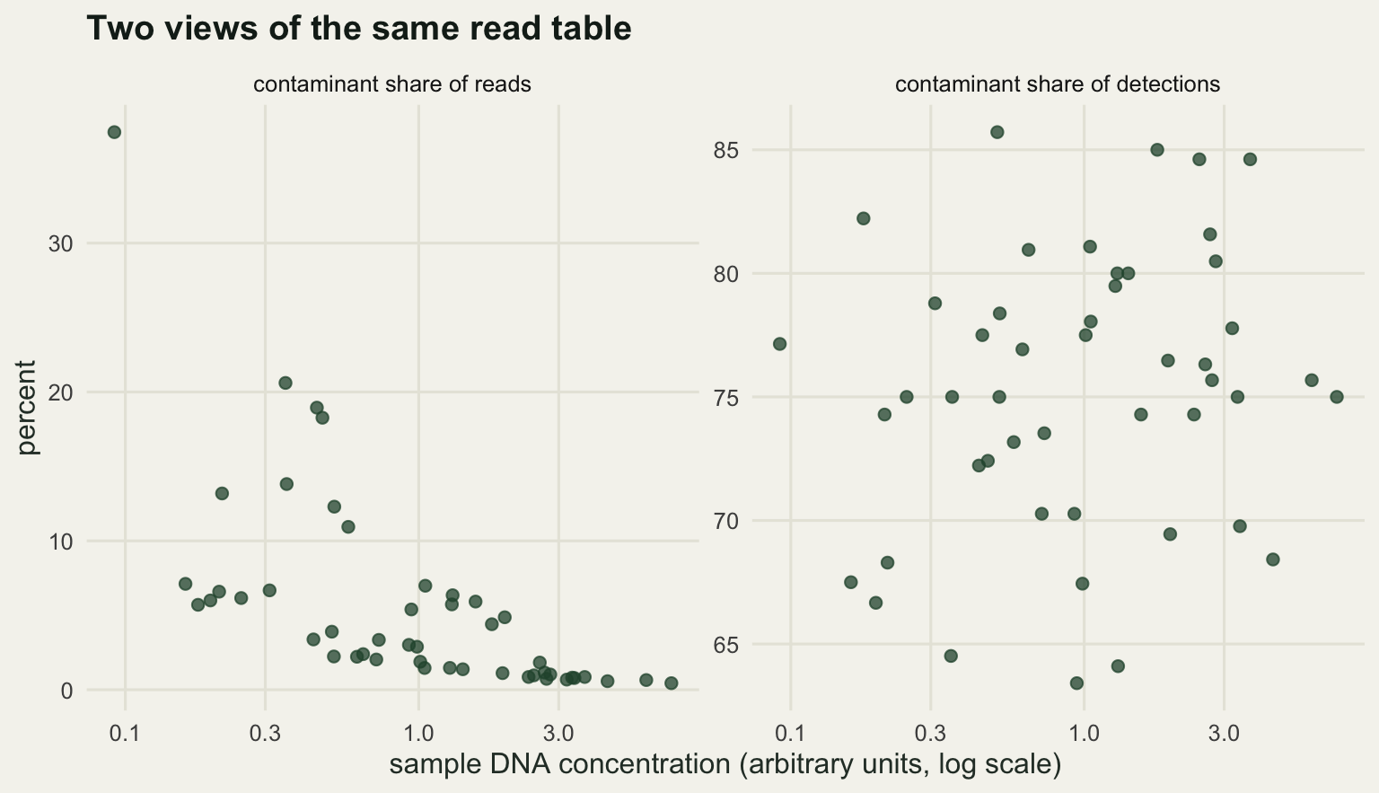
weakest <- which.min(conc_s); strongest <- which.max(conc_s)
print(round(c(reads_share_weakest = 100 * share_reads[weakest],
              reads_share_strongest = 100 * share_reads[strongest],
              det_share_weakest = 100 * share_det[weakest],
              det_share_strongest = 100 * share_det[strongest],
              det_share_lo = 100 * min(share_det)), 2))
reads_share_weakest reads_share_strongest det_share_weakest
37.45 0.44 77.14
det_share_strongest det_share_lo
75.00 63.41 The left panel is the pattern every reagent contamination method keys on: a fixed mass of contaminant DNA is a large share of a small extract and a small share of a large one, so the contaminant read share falls from 37.45 per cent in the weakest sample to 0.44 per cent in the strongest. The right panel does not fall at all: 75.00 per cent of the detections in the strongest sample were still created by contamination, and no sample in the run drops below 63.41 per cent.
Four rules, each swept
The rules below are the ones in common use. The first two work on a single cell, the third uses the blanks, and the fourth is a taxon-level test in the style of the decontam package: a frequency test asking whether a sequence’s relative abundance falls as sample DNA concentration rises, which is the signature of a constant contaminant mass, and a prevalence test asking whether it is more often present in blanks than in samples, combined by Fisher’s method.
Sensitivity is the share of real detections kept, specificity the share of false detections removed, both over the cells that are non-zero in the raw table. Each rule is swept across its tuning parameter, so the comparison is between rules at their best rather than at whatever settings happen to be conventional.
score <- function(keep) {
  c(sens = sum(keep & nz & truth) / n_real,
    spec = 1 - sum(keep & nz & !truth) / n_false,
    lost = sum(!keep & nz & truth),
    kept_false = sum(keep & nz & !truth))
}
best <- function(res, grd) {
  jj <- res[, "sens"] + res[, "spec"] - 1
  i <- which.max(jj)
  c(par = grd[i], res[i, ], youden = jj[i])
}

abs_grid <- unique(round(exp(seq(log(1), log(4000), length.out = 45))))
res_a <- t(sapply(abs_grid, function(a) score(tab >= a)))

rel_grid <- exp(seq(log(1e-6), log(0.08), length.out = 45))
relm <- sweep(tab, 2, tot_j, "/")
res_b <- t(sapply(rel_grid, function(f) score(relm >= f & nz)))

bmax <- apply(blk, 1, max)
mult_grid <- c(0, exp(seq(log(0.02), log(80), length.out = 44)))
res_c <- t(sapply(mult_grid, function(m) score(tab > m * bmax)))

print(c(grid_points_each = length(abs_grid), blank_max_total = sum(bmax)))
grid_points_each blank_max_total
40 18244 The frequency test compares two fixed-slope models for a taxon’s log relative abundance against log DNA concentration: slope minus one, which is what a constant contaminant mass gives, against slope zero, which is what a genuine constituent of the sample gives. The variance ratio between the two residual sums of squares is the test statistic.
freq_p <- rep(1, n_taxa); prev_p <- rep(1, n_taxa)
for (i in 1:n_taxa) {
  k <- tab[i, ] > 0
  if (sum(k) >= 4) {
    y <- log10(tab[i, k] / tot_j[k]); x <- log10(conc_s[k])
    ss_c <- sum((y + x - mean(y + x))^2)
    ss_n <- sum((y - mean(y))^2)
    dk <- sum(k) - 1
    freq_p[i] <- pf(ss_n / max(ss_c, 1e-12), dk, dk, lower.tail = FALSE)
  }
  prev_p[i] <- fisher.test(matrix(c(sum(blk[i, ] > 0), n_blank - sum(blk[i, ] > 0),
                                    sum(tab[i, ] > 0), n_samp - sum(tab[i, ] > 0)), 2),
                           alternative = "greater")$p.value
}
comb_p <- pchisq(-2 * (log(pmax(freq_p, 1e-300)) + log(pmax(prev_p, 1e-300))), 4,
                 lower.tail = FALSE)
p_grid <- c(exp(seq(log(1e-14), log(0.9), length.out = 44)), 1)
res_d <- t(sapply(p_grid, function(p) score(nz & !(comb_p < p))))

print(signif(c(freq_p_reagent = freq_p[reag_taxa]), 3))
freq_p_reagent1 freq_p_reagent2 freq_p_reagent3 freq_p_reagent4 freq_p_reagent5
9.07e-22 2.35e-20 9.21e-02 4.70e-06 4.83e-09 print(signif(c(min_prevalence_p = min(prev_p), taxa_prev_p_under_half = sum(prev_p < 0.5)), 3)) min_prevalence_p taxa_prev_p_under_half
0.265 2.000 print(c(flagged_at_default = sum(comb_p < 0.1),
reagent_taxa_flagged = sum(comb_p[reag_taxa] < 0.1),
false_kept = sum((nz & !(comb_p < 0.1)) & nz & !truth))) flagged_at_default reagent_taxa_flagged false_kept
4 4 1245 The prevalence test is dead on arrival in this run. Its smallest p-value across 60 taxa is 0.265, because index hopping puts nearly every sequence into nearly every library including the blanks, so being present in a blank carries no information. The whole taxon-level score is the frequency test, which is a useful thing to know before running it on a run with pervasive tag jumping.
b_a <- best(res_a, abs_grid); b_b <- best(res_b, rel_grid)
b_c <- best(res_c, mult_grid); b_d <- best(res_d, p_grid)
print(round(rbind(absolute = b_a, relative = b_b,
                  blank_max = b_c, frequency = b_d), 5))
par sens spec lost kept_false youden
absolute 36.00000 0.89778 0.83200 46 231 0.72978
relative 0.00037 0.95111 0.79709 22 279 0.74820
blank_max 0.78098 0.70000 0.75927 135 331 0.45927
frequency 0.00000 0.99333 0.06764 3 1282 0.06097mk <- function(res, nm) data.frame(spec = res[, "spec"], sens = res[, "sens"], rule = nm)
df_roc <- rbind(mk(res_a, "absolute reads"), mk(res_b, "relative abundance"),
mk(res_c, "blank maximum"), mk(res_d, "frequency test"))
df_pt <- data.frame(spec = c(b_a["spec"], b_b["spec"], b_c["spec"], b_d["spec"]),
sens = c(b_a["sens"], b_b["sens"], b_c["sens"], b_d["sens"]),
rule = c("absolute reads", "relative abundance",
"blank maximum", "frequency test"))
pal4 <- c("absolute reads" = te_pal$forest, "relative abundance" = te_pal$green,
"blank maximum" = te_pal$clay, "frequency test" = te_pal$gold)
ggplot(df_roc, aes(spec, sens, colour = rule)) +
geom_path(linewidth = 0.9) +
geom_point(data = df_pt, size = 3.4, shape = 18) +
scale_colour_manual(values = pal4) +
labs(x = "specificity (false detections removed)",
y = "sensitivity (real detections kept)") +
ggtitle("Filtering rules swept across their tuning parameters") +
theme_te()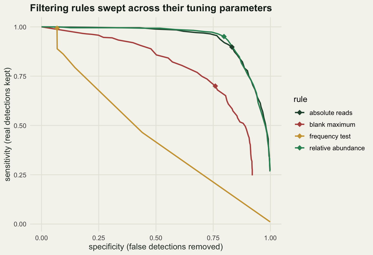
The two per-cell thresholds trace almost the same curve. That is the first surprise: library depth varies by a factor of 13.19 in this run, which is the situation a relative threshold exists to handle, and converting counts to proportions buys nothing measurable. At their best settings the absolute rule keeps 0.89778 of the real detections and removes 0.832 of the false ones at 36 reads, while the relative rule keeps 0.95111 and removes 0.79709 at 0.037 per cent of the sample total. They are two points on one curve, not two rules.
The blank maximum rule is worse everywhere on this plot, and the frequency test is not on the plot in any useful sense: at its best it flags 2 taxa and reaches a specificity of 0.06764, because a taxon-level rule can only remove the cells of taxa it deletes entirely. At the conventional cut of 0.1 it flags 4 taxa, all 4 of them real reagent contaminants, and still leaves 1245 false detections standing. Scored as a general-purpose filter it looks useless, which is the wrong way to score it.
Which rule catches which source
Every false detection has a dominant source, so the rules can be scored source by source. This is where the frequency test stops looking useless and the read thresholds stop looking sufficient.
c_x <- reads_cross[, samp_j]; c_g <- reads_reag[, samp_j]; c_h <- reads_hop[, samp_j]
src <- ifelse(c_x >= c_g & c_x >= c_h, 1L, ifelse(c_g >= c_h, 2L, 3L))
fc <- nz & !truth
keeps <- list("absolute reads" = tab >= b_a["par"],
              "relative abundance" = relm >= b_b["par"] & nz,
              "blank maximum" = tab > b_c["par"] * bmax,
              "frequency test" = nz & !(comb_p < b_d["par"]))
src_nm <- c("cross-contamination", "reagent", "index hopping")
sbs <- sapply(1:3, function(s)
  sapply(keeps, function(k) 1 - sum(k & fc & src == s) / sum(fc & src == s)))
colnames(sbs) <- src_nm
print(round(sbs, 3))
cross-contamination reagent index hopping
absolute reads 0.700 0.108 0.983
relative abundance 0.605 0.042 0.967
blank maximum 0.650 0.964 0.749
frequency test 0.000 0.560 0.000print(c(cells_cross = sum(fc & src == 1), cells_reagent = sum(fc & src == 2),
cells_hopping = sum(fc & src == 3))) cells_cross cells_reagent cells_hopping
220 166 989 df_tile <- data.frame(rule = rep(rownames(sbs), 3),
source = rep(src_nm, each = 4),
spec = as.vector(sbs))
df_tile$rule <- factor(df_tile$rule, levels = rev(rownames(sbs)))
df_tile$source <- factor(df_tile$source, levels = src_nm)
ggplot(df_tile, aes(source, rule, fill = spec)) +
geom_tile(colour = "#f5f4ee", linewidth = 1.5) +
geom_text(aes(label = sprintf("%.2f", spec)), colour = te_pal$ink, size = 4.2) +
scale_fill_gradient(low = te_pal$paper, high = te_pal$sage, limits = c(0, 1)) +
labs(x = NULL, y = NULL, fill = "specificity") +
ggtitle("No rule removes all three sources") +
theme_te()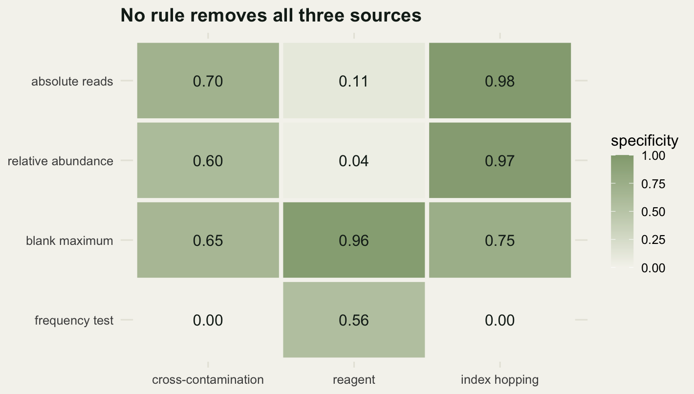
The pattern is clean. The two read thresholds remove 0.983 and 0.967 of the hopped detections, which are individually tiny, and 0.7 and 0.605 of the cross-contamination, but they remove little of the reagent contamination: 0.108 and 0.042. The blank maximum rule inverts that, taking out 0.964 of the reagent cells. The frequency test removes 0.56 of the reagent cells and, by construction, nothing else at all.
Why a read threshold cannot see reagent contamination is worth being precise about, because the usual explanation is half right. A fixed contaminant mass is a large fraction of a weak extract, so in read space it is large both absolutely and relatively there, and splitting the reagent cells by sample DNA concentration shows both threshold rules failing in the lower half of the range.
qb <- as.integer(cut(conc_s, quantile(conc_s, c(0, .25, .5, .75, 1)), include.lowest = TRUE))
qmat <- matrix(rep(qb, each = n_taxa), n_taxa, n_samp)
byq <- sapply(1:4, function(q) sapply(keeps, function(k)
  1 - sum(k & fc & src == 2 & qmat == q) / sum(fc & src == 2 & qmat == q)))
colnames(byq) <- paste0("Q", 1:4)
print(round(byq, 3))
Q1 Q2 Q3 Q4
absolute reads 0.000 0.000 0.089 0.318
relative abundance 0.000 0.000 0.000 0.159
blank maximum 0.850 1.000 1.000 1.000
frequency test 0.575 0.595 0.533 0.545print(round(100 * sapply(1:4, function(q) sum(c_g[, qb == q]) / sum(tab[, qb == q])), 3))[1] 5.298 2.101 1.036 0.455In the lowest concentration quartile the reagent sequences take 5.298 per cent of the reads and both threshold rules remove exactly none of them; in the top quartile they take 0.455 per cent and the absolute rule removes 0.318 of them. The only thing that separates a constant contaminant mass from a real constituent is its behaviour across the concentration gradient, and a per-cell threshold has no access to that gradient. It is a property of a taxon across samples, not of a cell.
Index hopping and the blank threshold need the opposite kind of care. The rule appears to remove 0.749 of the hopped cells at its tuned multiplier, but the blanks in this run sat on the plate and picked up cross-contamination from their neighbours, which inflated their maxima for exactly the abundant sequences that hopping also targets. Re-simulating the blanks as if they had been handled away from the plate, so that they see only the reagents and the flow cell, removes that accident.
blk2 <- matrix(0, n_taxa, n_blank)
for (b in 1:n_blank) {
  j <- blank_j[b]
  tot <- sum(mass_reag[, j]) + sum(mass_hop[, j])
  blk2[, b] <- rpois(n_taxa, depth_w[j] * (mass_reag[, j] + mass_hop[, j]) / tot)
}
bmax2 <- apply(blk2, 1, max)
spec_src <- function(keep) sapply(1:3, function(s)
  1 - sum(keep & fc & src == s) / sum(fc & src == s))
print(round(c(on_plate = spec_src(tab > bmax), off_plate = spec_src(tab > bmax2)), 3))
on_plate1 on_plate2 on_plate3 off_plate1 off_plate2 off_plate3
0.673 0.976 0.797 0.127 1.000 0.430 top6 <- order(-hop_prof)[1:6]
print(rbind(sample_hop_reads = apply(reads_hop[top6, samp_j], 1, median),
blank_hop_reads = apply(reads_hop[top6, blank_j], 1, median),
off_plate_threshold = bmax2[top6])) [,1] [,2] [,3] [,4] [,5] [,6]
sample_hop_reads 31.5 14.0 14 8.5 7.5 6
blank_hop_reads 3.0 1.5 2 0.5 1.0 1
off_plate_threshold 18.0 13.0 8 9.0 2.0 5print(round(c(depth_ratio = mean(depth_w[samp_j]) / mean(depth_w[blank_j]),
hop_cells_retained = sum((tab > bmax2) & fc & src == 3),
hop_cells_total = sum(fc & src == 3)), 2)) depth_ratio hop_cells_retained hop_cells_total
9.99 564.00 989.00 Take the standard version of the rule, delete anything at or below the maximum count in the negative controls. With the on-plate blanks it removes 0.797 of the hopped cells; with blanks that only see the sequencing it removes 0.43 and leaves 564 of 989 in place. The mechanism is a scale mismatch: hopping delivers reads in proportion to a library’s own depth, the blanks here were sequenced 9.99 times more shallowly than the samples, so the counts they show for a hopped sequence are an order of magnitude too small. The run’s most abundant sequence contributes a median of 31.5 hopped reads to a sample and 3 to a blank. A blank cannot calibrate a process that scales with the run unless it was sequenced like a sample.
The on-plate blanks did better, but by accident rather than by design: an argument for blanks that ride the plate, not an argument that the rule understands hopping.
What filtering costs the answer
Sensitivity and specificity are not what a diet study reports. Frequency of occurrence is: the proportion of samples in which each prey taxon was detected. The truth is known here, so the same quantity can be computed on the true presence matrix, the raw table, and each filtered table.
foo_true <- rowMeans(truth)
mae_of <- function(keep) 100 * mean(abs(rowMeans(keep & nz) - foo_true))
tabs <- c(list("raw table" = nz), keeps)
m4 <- t(sapply(tabs, function(k)
  c(foo_error_pp = mae_of(k), mean_richness = mean(colSums(k & nz)))))
m4 <- cbind(m4, youden = c(NA, b_a["youden"], b_b["youden"], b_c["youden"], b_d["youden"]))
print(round(m4, 3))
foo_error_pp mean_richness youden
raw table 47.743 38.021 NA
absolute reads 7.535 13.229 0.730
relative abundance 9.271 14.729 0.748
blank maximum 15.069 13.458 0.459
frequency test 44.618 36.021 0.061print(round(c(true_mean_richness = mean(colSums(truth))), 3))true_mean_richness
9.375 both <- keeps[["absolute reads"]] & keeps[["blank maximum"]]
print(round(c(score(both), youden = sum(score(both)[1:2]) - 1,
foo_error_pp = mae_of(both),
mean_richness = mean(colSums(both & nz))), 4)) sens spec lost kept_false youden
0.6778 0.9745 145.0000 35.0000 0.6523
foo_error_pp mean_richness
4.9306 7.0833 mae_a <- sapply(abs_grid, function(a) mae_of(tab >= a))
print(round(c(foo_best_threshold = abs_grid[which.min(mae_a)],
foo_best_error = min(mae_a),
foo_best_sens = score(tab >= abs_grid[which.min(mae_a)])["sens"],
youden_threshold_error = mae_of(tab >= b_a["par"])), 4)) foo_best_threshold foo_best_error foo_best_sens.sens
196.0000 5.7986 0.7044
youden_threshold_error
7.5347 Mean absolute error in frequency of occurrence, in percentage points, can rank the rules differently from the Youden index, and where it does the disagreement is not a rounding artefact. Here the relative threshold has the better classifier score, 0.7482 against 0.72978, and the worse ecological answer, 9.271 percentage points against 7.535. The reason is that false detections outnumber real ones three to one in this table, and the Youden index divides each error by the count of detections of its own kind, so it prices an error on a real detection at three times an error on a false one, while the frequency estimate prices them equally, cell for cell.
The same effect shows up inside a single rule. Sweeping the absolute threshold for frequency error instead of for the Youden index moves the optimum from 36 reads to 196 reads, cutting the error from 7.5347 to 5.7986 percentage points while dropping sensitivity to 0.7044. And applying the absolute and blank maximum rules together gives a worse classifier than the absolute rule alone, 0.6523 against 0.72978, with a frequency error of 4.9306 percentage points, lower than either read threshold on its own. A rule can be a better classifier and a worse analysis, and if the report is a frequency of occurrence then the analysis is what should be tuned.
None of the filtered tables recovers the true mean richness of 9.375 taxa per sample. The best per-cell rules leave 13.229 and 14.729, the combined rule overshoots in the other direction at 7.083. Filtering moves the bias; it does not remove it.
How many blanks are enough
The blank-based rules depend on an estimate made from a handful of libraries, so the number of blanks controls both the precision of that estimate and the variability it puts into the filtered table. The comparison point is the variability the sequencing itself contributes, computed by redrawing the sample table from the same Poisson means with the threshold held fixed. Below that floor, more blanks cannot buy anything.
set.seed(4041)
blank_mass <- rowMeans(mass_reag[, blank_j] + mass_cross[, blank_j] + mass_hop[, blank_j])
blank_lam <- 6000 * blank_mass / sum(blank_mass)
big <- blank_lam >= 1
n_rep <- 400
nb_grid <- c(1, 2, 3, 4, 6, 8, 12, 16)
mult_use <- b_c["par"]
out5 <- NULL
for (nb in nb_grid) {
  em <- matrix(0, n_rep, n_taxa)
  kf_mn <- lo_mn <- lo_mx <- thr_mx <- numeric(n_rep)
  for (r in 1:n_rep) {
    bb <- matrix(rpois(n_taxa * nb, rep(blank_lam, nb)), n_taxa, nb)
    em[r, ] <- rowMeans(bb)
    tmx <- apply(bb, 1, max)
    k_mn <- tab > mult_use * em[r, ]
    k_mx <- tab > mult_use * tmx
    kf_mn[r] <- sum(k_mn & nz & !truth); lo_mn[r] <- sum(!k_mn & nz & truth)
    lo_mx[r] <- sum(!k_mx & nz & truth); thr_mx[r] <- sum(tmx)
  }
  rse <- apply(em[, big], 2, sd) / apply(em[, big], 2, mean)
  out5 <- rbind(out5, c(blanks = nb, rel_se = median(rse),
                        sd_false_kept = sd(kf_mn), sd_real_lost = sd(lo_mn),
                        max_rule_lost = mean(lo_mx), max_threshold = mean(thr_mx)))
}
print(round(out5, 4))
blanks rel_se sd_false_kept sd_real_lost max_rule_lost max_threshold
[1,] 1 0.2802 28.2415 1.2015 87.2000 6001.505
[2,] 2 0.2130 20.5835 0.9574 88.6250 6180.837
[3,] 3 0.1691 19.8629 0.9154 89.1600 6274.517
[4,] 4 0.1385 18.4646 0.8492 89.6175 6338.385
[5,] 6 0.1196 15.1790 0.8462 90.0825 6411.120
[6,] 8 0.0989 14.9800 0.8694 90.4125 6469.597
[7,] 12 0.0857 12.0148 0.8727 90.9025 6539.390
[8,] 16 0.0699 12.4104 0.8419 91.4925 6587.132thr_fix <- mult_use * blank_lam
mm <- (mass_real + mass_reag + mass_cross + mass_hop)[, samp_j]
lam_s <- sweep(mm, 2, colSums(mm), "/") %*% diag(depth_w[samp_j])
kf_s <- numeric(n_rep)
for (r in 1:n_rep) {
t2 <- matrix(rpois(length(lam_s), lam_s), nrow(lam_s))
kf_s[r] <- sum((t2 > thr_fix) & (t2 > 0) & !truth)
}
print(round(c(sequencing_floor_sd = sd(kf_s), taxa_estimated = sum(big)), 3))sequencing_floor_sd taxa_estimated
11.726 35.000 The relative standard error of the per-taxon contaminant intensity falls the way a Poisson mean estimated from independent replicates should: 0.2802 with one blank, 0.1385 with four, 0.0699 with sixteen. The number that decides the design is the next column. The blank-induced standard deviation in the count of false detections that survive the filter is 28.2415 cells with one blank and 18.4646 with four, against a sequencing floor of 11.726 cells that no number of blanks can reduce. By eight blanks the blank contribution is 14.98 and the two sources are comparable; past twelve, adding blanks changes the total variability by less than the run-to-run Poisson noise already present.
panel_lv2 <- c("relative SE of contaminant intensity",
               "SD of surviving false detections (cells)")
df_b <- data.frame(blanks = rep(out5[, "blanks"], 2),
                   val = c(out5[, "rel_se"], out5[, "sd_false_kept"]),
                   panel = factor(rep(panel_lv2, each = nrow(out5)), levels = panel_lv2))
df_floor <- data.frame(panel = factor(panel_lv2[2], levels = panel_lv2), yy = sd(kf_s))
ggplot(df_b, aes(blanks, val)) +
  geom_line(colour = te_pal$forest, linewidth = 0.9) +
  geom_point(colour = te_pal$forest, size = 2.4) +
  geom_hline(data = df_floor, aes(yintercept = yy), linetype = "dashed",
             colour = te_pal$clay, linewidth = 0.8) +
  facet_wrap(~panel, scales = "free_y") +
  labs(x = "number of extraction blanks", y = NULL) +
  ggtitle("What extra blanks buy, and where they stop buying") +
  theme_te()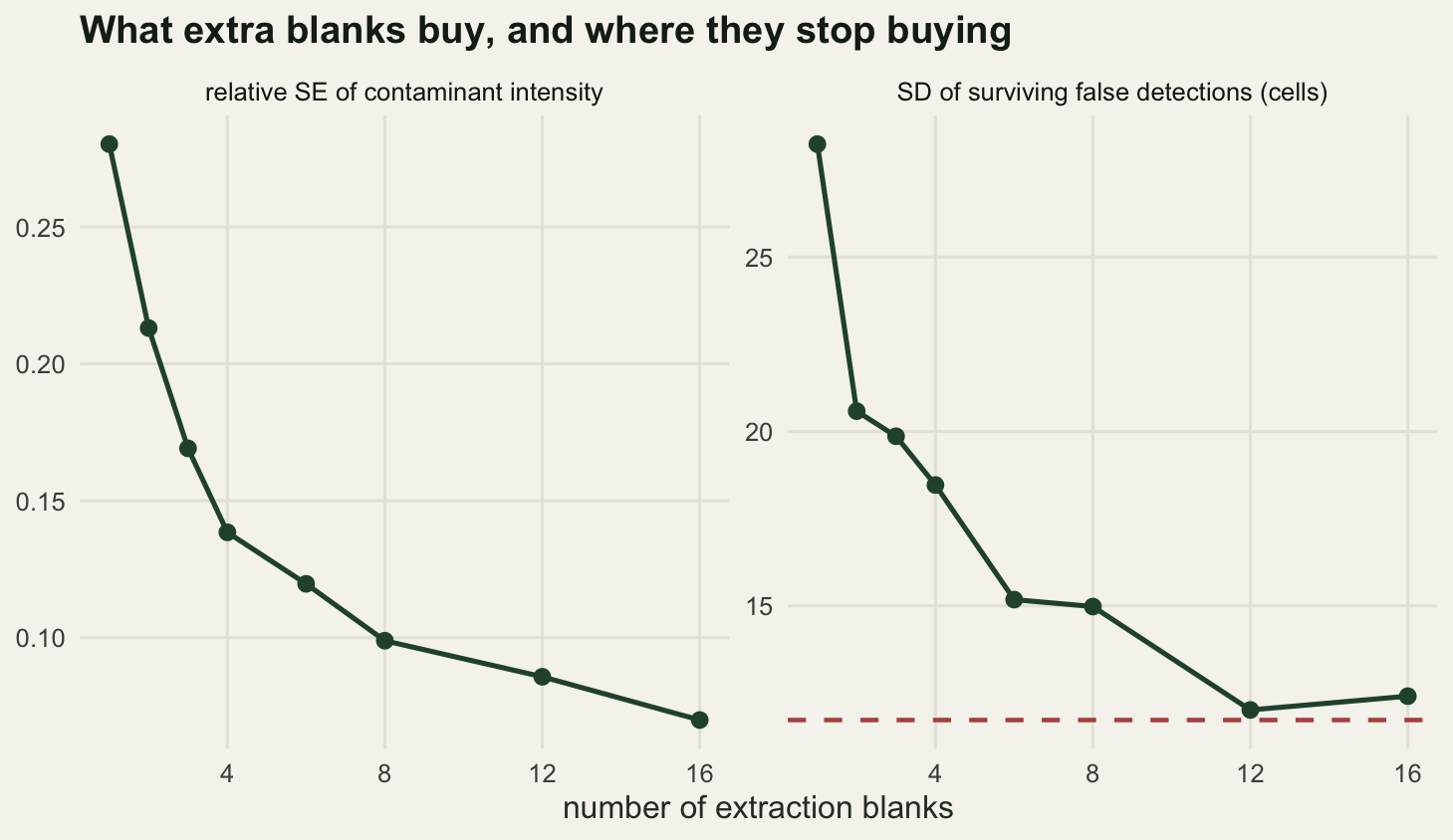
The last two columns of that sweep are a warning about how the rule is usually written. A threshold set at the maximum count across the blanks is not an estimate of anything: the maximum of more draws is larger, so the summed threshold grows from 6001.5 with one blank to 6587.1 with sixteen, and the real detections it destroys rise from 87.2 to 91.4925. The same written rule, applied to the same table, is a stricter filter in a study with more negative controls. A mean across blanks does not have this property, and it is what should be reported.
What none of these rules can do
Every rule here needs contamination to differ from signal in a way the data record. A count threshold needs contaminant cells to be smaller. A blank threshold needs the contaminant to reach the blank. A frequency test needs a concentration gradient wide enough for the slope to declare itself. When a taxon is both signal and contaminant in the same samples, every rule that fires on it deletes real detections too, and the simulator contains one such taxon on purpose.
print(round(c(true_occupancy = mean(truth[hard_i, ]),
              real_detections = sum(nz[hard_i, ] & truth[hard_i, ]),
              median_reads_present = median(tab[hard_i, truth[hard_i, ]]),
              share_of_all_real = 100 * sum(nz[hard_i, ] & truth[hard_i, ]) / n_real), 3))
true_occupancy real_detections median_reads_present
0.979 47.000 82.000
share_of_all_real
10.444 print(signif(c(frequency_p = freq_p[hard_i], combined_p = comb_p[hard_i]), 3))frequency_p combined_p
4.83e-09 9.74e-08 print(sapply(keeps, function(k) sum(k[hard_i, ] & truth[hard_i, ]))) absolute reads relative abundance blank maximum frequency test
41 47 2 47 Taxon 37 is a genuine prey item in 0.979 of the samples, always at low relative abundance, and it is also in the reagents. Its counts where it is genuinely present are a median of 82 reads, most of them contaminant. The frequency test is right about it in the sense it was designed for: the relative abundance does fall as the concentration rises, with a combined p-value of 9.74e-08, so the default cut flags it and every one of its 47 real detections is deleted, 10.444 per cent of all the real detections in the table. The blank maximum rule keeps 2 of the 47. The absolute threshold keeps 41 and can only do that because it also keeps the contaminant reads that inflated the counts in the first place.
No arrangement of thresholds recovers this taxon, because the information needed is not in the table. What would resolve it sits outside the data: blanks carrying a known amount of an exogenous spike so the contaminant mass is measured rather than inferred, a second marker the reagent contaminant does not amplify, or an independent observation of the diet. Failing those, the honest report is that the taxon’s status is undecided, not that it was removed.
That generalises. Deleting a taxon or a cell is a claim about the biology, made with a classifier whose error rates the reader cannot see. The rule and its threshold belong in the results with the numbers they produced: which rule, which parameter, how many cells and how many taxa went, and what the estimate looks like without them. A methods sentence about removing singletons and low-abundance reads hides a decision that moved the frequency of occurrence in this table by more than 40 percentage points.
Where to go next
The cluster’s last post, Checking a metabarcoding analysis, takes the filtered table forward and asks what can still be checked once the deletions are made: whether the rule that produced the table changes the answer, and which diagnostics survive the compositional constraint the first post established.
The practical summary is short. Run more than one rule, because they catch different sources. Sweep the parameter against the quantity you are going to report, not only against a classification score. Sequence the blanks like samples if they are meant to calibrate anything about the sequencing. And write the rule down.
References
Davis NM, Proctor DM, Holmes SP, Relman DA, Callahan BJ 2018 Microbiome 6:226 (10.1186/s40168-018-0605-2)
Salter SJ, Cox MJ, Turek EM, Calus ST, Cookson WO, Moffatt MF, Turner P, Parkhill J, Loman NJ, Walker AW 2014 BMC Biology 12:87 (10.1186/s12915-014-0087-z)
Schnell IB, Bohmann K, Gilbert MTP 2015 Molecular Ecology Resources 15(6):1289-1303 (10.1111/1755-0998.12402)
Taberlet P, Coissac E, Hajibabaei M, Rieseberg LH 2012 Molecular Ecology 21(8):1789-1793 (10.1111/j.1365-294X.2012.05542.x)
Ficetola GF, Taberlet P, Coissac E 2016 Molecular Ecology Resources 16(3):604-607 (10.1111/1755-0998.12508)
Costello M, Fleharty M, Abreu J, Farjoun Y, Ferriera S, Holmes L, Granger B, Green L, Howd T, Mason T, Vicente G, Dasilva M, Brodeur W, DeSmet T, Dodge S, Lennon NJ, Gabriel S 2018 BMC Genomics 19:332 (10.1186/s12864-018-4703-0)