library(ggplot2)

te_pal <- list(forest = "#275139", green = "#2f8f63", sage = "#93a87f",
               clay = "#b5534e", gold = "#cda23f", line = "#dad9ca",
               ink = "#16241d", paper = "#f5f4ee")

theme_te <- function() {
  theme_minimal(base_size = 12) +
    theme(panel.grid.minor = element_blank(),
          panel.grid.major = element_line(colour = "#e7e6dc"),
          plot.background = element_rect(fill = "#f5f4ee", colour = NA),
          panel.background = element_rect(fill = "#f5f4ee", colour = NA),
          plot.title = element_text(face = "bold", colour = te_pal$ink),
          axis.title = element_text(colour = "#2c3a31"))
}False positives in eDNA surveys
R
eDNA
occupancy
imperfect detection
ecology tutorial
ggplot2
A contaminated PCR replicate looks exactly like a rare detection. Fit the false-positive mixture for eDNA occupancy in R and measure what field blanks buy.
The three-level eDNA model assumed that a positive PCR replicate means target DNA was in the tube. Field gear carries DNA between sites, a pipette tip touches the wrong rack, indices jump between libraries on the same run, and a primer designed for one species amplifies its congener. Any of these produces a positive replicate from water that never held the target.
In occupancy language the replicate-level detection becomes a two-component mixture: probability p11 of a positive when the sample really carries DNA, probability p10 of a positive when it does not. The difficulty is not writing that likelihood down. It is that a rare true detection and a contamination event produce identical data, so the survey has to be designed to tell them apart. This tutorial measures the bias from ignoring a contamination rate of two per cent, fits the mixture, measures what it costs, measures what negative controls buy, and scores the replicate-count rule that field protocols use instead.
The Royle and Link version of this mixture, at the visit level in an ordinary occupancy model, is built in the false positives tutorial and assumed here. What follows is the eDNA case: contamination entering at the replicate level inside a three-level hierarchy.
The likelihood, with contamination put back
A site is occupied with probability psi. Given occupancy, each water sample carries detectable DNA with probability theta. Each PCR replicate of a sample amplifies with probability p11 if that sample carries DNA and p10 if it does not. At an unoccupied site every sample is DNA-free, so every one of its replicates amplifies with probability p10, and the site contributes the product of those binomial terms alone.
sim_edna <- function(n_site, n_samp, n_rep, psi, theta, p11, p10) {
  z <- rbinom(n_site, 1, psi)
  occ <- matrix(rbinom(n_site * n_samp, 1, theta), n_site, n_samp) * z
  matrix(rbinom(length(occ), n_rep, ifelse(occ == 1, p11, p10)), n_site, n_samp)
}

nll_full <- function(par, y, n_rep, blanks = NULL) {
  psi <- plogis(par[1])
  theta <- plogis(par[2])
  p10 <- plogis(par[3])
  gap <- plogis(par[4])
  p11 <- p10 + (1 - p10) * gap
  d1 <- theta * dbinom(y, n_rep, p11) + (1 - theta) * dbinom(y, n_rep, p10)
  l1 <- rowSums(log(d1))
  l0 <- rowSums(dbinom(y, n_rep, p10, log = TRUE))
  mx <- pmax(l1, l0)
  ll <- sum(mx + log(psi * exp(l1 - mx) + (1 - psi) * exp(l0 - mx)))
  if (!is.null(blanks)) ll <- ll + sum(dbinom(blanks, n_rep, p10, log = TRUE))
  if (!is.finite(ll)) return(1e10)
  -ll
}

nll_naive <- function(par, y, n_rep) {
  psi <- plogis(par[1])
  theta <- plogis(par[2])
  p11 <- plogis(par[3])
  d1 <- theta * dbinom(y, n_rep, p11) + (1 - theta) * (y == 0)
  l1 <- rowSums(log(d1))
  l0 <- ifelse(rowSums(y) == 0, 0, -Inf)
  mx <- pmax(l1, l0)
  ll <- sum(mx + log(psi * exp(l1 - mx) + (1 - psi) * exp(l0 - mx)))
  if (!is.finite(ll)) return(1e10)
  -ll
}

par_full <- function(par) {
  p10 <- plogis(par[3])
  c(psi = plogis(par[1]), theta = plogis(par[2]),
    p11 = p10 + (1 - p10) * plogis(par[4]), p10 = p10)
}

se_full <- function(fit) {
  par <- fit$par
  p10 <- plogis(par[3])
  gap <- plogis(par[4])
  jac <- matrix(0, 4, 4)
  jac[1, 1] <- plogis(par[1]) * (1 - plogis(par[1]))
  jac[2, 2] <- plogis(par[2]) * (1 - plogis(par[2]))
  jac[3, 3] <- (1 - gap) * p10 * (1 - p10)
  jac[3, 4] <- (1 - p10) * gap * (1 - gap)
  jac[4, 3] <- p10 * (1 - p10)
  sqrt(diag(jac %*% solve(fit$hessian) %*% t(jac)))
}

se_naive <- function(fit) {
  p <- plogis(fit$par)
  vc <- try(solve(fit$hessian), silent = TRUE)
  if (inherits(vc, "try-error")) return(rep(NA_real_, 3))
  s <- suppressWarnings(sqrt(diag(diag(p * (1 - p)) %*% vc %*% diag(p * (1 - p)))))
  ifelse(is.finite(s) & s > 1e-8, s, NA_real_)
}

fit_full <- function(y, n_rep, blanks = NULL, start = c(0, 0, -3, 0.5)) {
  optim(start, nll_full, y = y, n_rep = n_rep, blanks = blanks, method = "BFGS",
        hessian = TRUE, control = list(maxit = 500))
}

fit_naive <- function(y, n_rep) {
  optim(c(0, 0, 0.5), nll_naive, y = y, n_rep = n_rep, method = "BFGS",
        hessian = TRUE, control = list(maxit = 500))
}
Two details there matter. All four parameters sit on the logit scale, but p11 is built as p10 plus a fraction of the room above it, which forces p11 above p10: the likelihood is otherwise symmetric under swapping the two components and their labels. The site term uses a log-sum-exp so that a site with forty near-impossible replicates does not silently become a zero.
Simulating a survey, and counting the accidents
Two parameter sets follow. In the first the two components are far apart: amplification usually succeeds when DNA is present and contamination is rare. In the second the target is scarce and the background dirty, so a DNA-bearing sample and a contaminated one look much more alike.
n_site <- 150
n_samp <- 5
n_rep <- 8
truth_a <- c(psi = 0.5, theta = 0.5, p11 = 0.7, p10 = 0.02)
truth_b <- c(psi = 0.5, theta = 0.5, p11 = 0.30, p10 = 0.15)

cat("sites:", n_site, " samples per site:", n_samp,
    " replicates per sample:", n_rep,
    " replicates per site:", n_samp * n_rep, "\n")
sites: 150 samples per site: 5 replicates per sample: 8 replicates per site: 40 print(rbind(separated = truth_a, overlapping = truth_b)) psi theta p11 p10
separated 0.5 0.5 0.7 0.02
overlapping 0.5 0.5 0.3 0.15cat("ratio of p11 to p10:", round(truth_a[3] / truth_a[4], 2),
"in the separated set and", round(truth_b[3] / truth_b[4], 2),
"in the overlapping set\n")ratio of p11 to p10: 35 in the separated set and 2 in the overlapping setsite_fp <- function(p10, n) 1 - (1 - p10)^n
cat("chance that an unoccupied site gives at least one positive replicate:",
round(site_fp(truth_a[4], n_samp * n_rep), 4), "separated,",
round(site_fp(truth_b[4], n_samp * n_rep), 4), "overlapping\n")chance that an unoccupied site gives at least one positive replicate: 0.5543 separated, 0.9985 overlappingcat("chance for a single unoccupied sample of", n_rep, "replicates:",
round(site_fp(truth_a[4], n_rep), 4), "\n")chance for a single unoccupied sample of 8 replicates: 0.1492 set.seed(511)
y_a <- sim_edna(n_site, n_samp, n_rep, truth_a[1], truth_a[2], truth_a[3],
truth_a[4])
cat("water samples:", n_site * n_samp, " field replicates in total:",
n_site * n_samp * n_rep, "\n")water samples: 750 field replicates in total: 6000 cat("sites with at least one positive replicate:",
round(mean(rowSums(y_a) > 0), 4), "\n")sites with at least one positive replicate: 0.7533 print(table(positives_per_sample = as.vector(y_a)))positives_per_sample
0 1 2 3 4 5 6 7 8
481 75 8 14 31 49 48 38 6 The false-positive line in that output is the whole problem in one number. A contamination rate of 0.02 sounds ignorable, but each site gets 40 replicates, and the chance that at least one of them comes up positive at an unoccupied site is 0.5543. Half the empty sites in this survey look occupied. The observed detection rate confirms it: 0.7533 of sites have a positive replicate somewhere, while only half of them are truly occupied.
The count table shows the one clue the data does offer. Of the 750 water samples, 481 gave no positive replicate at all; then come 75 samples with exactly one positive and a separate hump at four to seven positives. The isolated single positives are mostly contamination and the hump is real DNA. Nothing labels an individual sample, but the shapes of the two distributions differ, and that difference is what the mixture uses.
Fitting the model that assumes clean water
Set p10 to zero and refit. This is what almost every published eDNA occupancy analysis does.
fa_naive <- fit_naive(y_a, n_rep)
print(data.frame(parameter = c("psi", "theta", "p11"),
                 truth = as.vector(truth_a[1:3]),
                 estimate = round(plogis(fa_naive$par), 4),
                 se = round(se_naive(fa_naive), 4)), row.names = FALSE)
parameter truth estimate se
psi 0.5 0.7923 0.0380
theta 0.5 0.4542 0.0231
p11 0.7 0.5113 0.0109Occupancy comes back as 0.7923 when the truth is 0.5, with a standard error of 0.038, so the truth is more than seven standard errors away. The model has no way to explain a positive replicate except as real DNA, so every site that suffered a contamination event is recorded as occupied, and psi absorbs the 0.5543.
The other two parameters move in compensation. Sample-level occurrence falls to 0.4542 and the true-positive rate collapses to 0.5113 from 0.7, because the contaminated samples are being treated as DNA-bearing samples that happened to amplify once out of eight. The model is not merely imprecise; it has redistributed the signal across all three levels.
mech <- expand.grid(p10 = seq(0, 0.10, length.out = 121),
                    reps = c(8, 24, 40, 80))
mech$prob <- site_fp(mech$p10, mech$reps)
mech$series <- factor(paste(mech$reps, "replicates per site"),
                      levels = paste(c(8, 24, 40, 80), "replicates per site"))
mark <- data.frame(p10 = as.vector(truth_a[4]),
                   prob = site_fp(as.vector(truth_a[4]), n_samp * n_rep))

ggplot(mech, aes(p10, prob, colour = series)) +
  geom_line(linewidth = 0.9) +
  geom_point(data = mark, aes(p10, prob), inherit.aes = FALSE,
             colour = te_pal$ink, size = 2.8) +
  scale_colour_manual(values = c(te_pal$sage, te_pal$gold, te_pal$green,
                                 te_pal$forest), name = NULL) +
  labs(title = "Effort multiplies contamination as well as detection",
       subtitle = "dot: the design simulated here, five samples of eight replicates",
       x = "replicate-level false positive rate p10",
       y = "chance of at least one positive") +
  theme_te()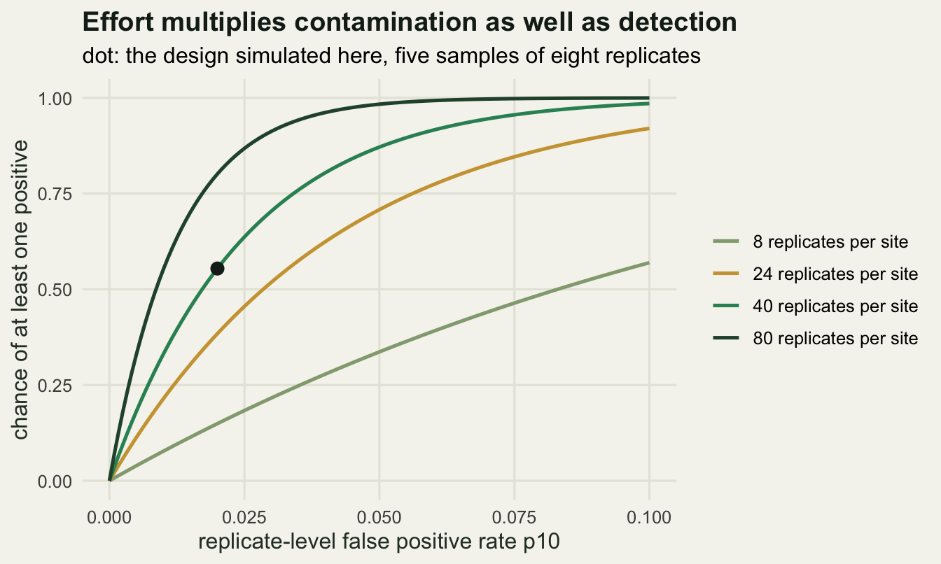
The shape of those curves is the practical point. Contamination is a per-replicate accident, so a survey that adds replicates to improve detection is also buying more chances to be fooled. Raising effort does not dilute a false positive problem; it concentrates it.
Fitting the mixture
Now estimate all four parameters.
fa_full <- fit_full(y_a, n_rep)
se_a <- se_full(fa_full)
print(data.frame(parameter = names(truth_a), truth = as.vector(truth_a),
                 estimate = round(par_full(fa_full$par), 4),
                 se = round(se_a, 4)), row.names = FALSE)
parameter truth estimate se
psi 0.50 0.4885 0.0423
theta 0.50 0.5127 0.0286
p11 0.70 0.6762 0.0124
p10 0.02 0.0195 0.0021cat("standard error of psi, mixture divided by p10 fixed at zero:",
round(se_a[1] / se_naive(fa_naive)[1], 4), "\n")standard error of psi, mixture divided by p10 fixed at zero: 1.1132 Every parameter comes back where it belongs: psi 0.4885, theta 0.5127, p11 0.6762 and p10 0.0195 against a true 0.02. Adding the fourth parameter widens the standard error of psi by a factor of 1.1132, from 0.038 to 0.0423. That is a small premium for removing a bias of nearly 0.3, and on this design the answer to “can you fit it” is simply yes.
Where the mixture stops working
The premium is small because the two components barely overlap: p11 is 35 times p10, so a DNA-bearing sample gives five or six positives out of eight and a contaminated one gives zero or one. Move the parameters together and that separation goes.
set.seed(513)
y_b <- sim_edna(n_site, n_samp, n_rep, truth_b[1], truth_b[2], truth_b[3],
                truth_b[4])
fb_naive <- fit_naive(y_b, n_rep)
fb_full <- fit_full(y_b, n_rep, start = c(0, 0, -2, 0))
se_b <- se_full(fb_full)
cat("p10 fixed at zero, overlapping design:",
    round(plogis(fb_naive$par), 4), "\n")
p10 fixed at zero, overlapping design: 1 1 0.189 print(data.frame(parameter = names(truth_b), truth = as.vector(truth_b),
estimate = round(par_full(fb_full$par), 4),
se = round(se_b, 4)), row.names = FALSE) parameter truth estimate se
psi 0.50 0.4788 0.1561
theta 0.50 0.8510 0.1618
p11 0.30 0.2599 0.0251
p10 0.15 0.1403 0.0149cat("standard error of psi, overlapping divided by separated:",
round(se_b[1] / se_a[1], 4), "\n")standard error of psi, overlapping divided by separated: 3.6909 The naive fit on this design does not fail gracefully, it fails completely: psi and theta both go to 1 and the true-positive rate settles at 0.189. With p10 at 0.15 the chance that an unoccupied site yields a positive replicate is 0.9985, so every site looks occupied and every sample looks like it held DNA. The estimator is pinned against its boundary, which is also why its standard errors are undefined.
The mixture lands at 0.4788 against a true 0.5 on this survey, but the standard error is 0.1561, a factor of 3.6909 wider than on the separated design. Repeating the whole fit on fresh surveys shows what is actually going on.
study <- function(truth, n_it, seed, start) {
  set.seed(seed)
  out <- matrix(NA_real_, n_it, 8)
  for (i in seq_len(n_it)) {
    yy <- sim_edna(n_site, n_samp, n_rep, truth[1], truth[2], truth[3], truth[4])
    bb <- rbinom(50, n_rep, truth[4])
    out[i, 1:4] <- par_full(optim(start, nll_full, y = yy, n_rep = n_rep,
      method = "BFGS", control = list(maxit = 500))$par)
    out[i, 5:8] <- par_full(optim(start, nll_full, y = yy, n_rep = n_rep,
      blanks = bb, method = "BFGS", control = list(maxit = 500))$par)
  }
  out
}

study_a <- study(truth_a, 200, 517, c(0, 0, -3, 0.5))
study_b <- study(truth_b, 200, 518, c(0, 0, -2, 0))
cat("separated design, 200 fits: mean psi", round(mean(study_a[, 1]), 4),
    " sd", round(sd(study_a[, 1]), 4),
    " correlation of psi with p10", round(cor(study_a[, 1], study_a[, 4]), 4),
    "\n")
separated design, 200 fits: mean psi 0.5022 sd 0.0426 correlation of psi with p10 0.12 cat("overlapping design, 200 fits: mean psi", round(mean(study_b[, 1]), 4),
" sd", round(sd(study_b[, 1]), 4),
" correlation of psi with p10", round(cor(study_b[, 1], study_b[, 4]), 4),
"\n")overlapping design, 200 fits: mean psi 0.5429 sd 0.2241 correlation of psi with p10 -0.6794 Across 200 simulated surveys the separated design gives a mean psi of 0.5022 and a correlation between the psi and p10 estimates of 0.12, which is nothing. The overlapping design gives a mean of 0.5429, so a small upward bias survives, a standard deviation of 0.2241, and a correlation of -0.6794. That negative correlation is the weak identifiability made visible: a survey that happens to look slightly dirty gets a higher p10 and a lower psi, because the likelihood is close to indifferent between “this site is occupied and amplification is unreliable” and “this site is empty and the lab is dirty”.
So identifiability here is not a property of the model. It is a property of the design, and the quantity that decides it is how far p11 sits above p10 relative to the number of replicates.
What blanks buy, measured
The fix is information from outside the survey. Add 50 blank samples known to come from water with no target, each run through the same eight replicates, and their positive counts estimate p10 directly.
set.seed(515)
blank_a <- rbinom(50, n_rep, truth_a[4])
set.seed(516)
blank_b <- rbinom(50, n_rep, truth_b[4])
cat("blank samples:", length(blank_a), " blank replicates:",
    length(blank_a) * n_rep, " positives:", sum(blank_a), "separated,",
    sum(blank_b), "overlapping, an apparent rate of",
    round(sum(blank_b) / (length(blank_b) * n_rep), 4), "\n")
blank samples: 50 blank replicates: 400 positives: 9 separated, 71 overlapping, an apparent rate of 0.1775 fa_cal <- fit_full(y_a, n_rep, blanks = blank_a)
fb_cal <- fit_full(y_b, n_rep, blanks = blank_b, start = c(0, 0, -2, 0))
print(data.frame(design = rep(c("separated", "overlapping"), each = 4),
parameter = rep(names(truth_a), 2),
estimate = round(c(par_full(fa_cal$par),
par_full(fb_cal$par)), 4),
se = round(c(se_full(fa_cal), se_full(fb_cal)), 4)),
row.names = FALSE) design parameter estimate se
separated psi 0.4885 0.0423
separated theta 0.5126 0.0286
separated p11 0.6763 0.0124
separated p10 0.0198 0.0020
overlapping psi 0.3597 0.1210
overlapping theta 0.8718 0.2121
overlapping p11 0.2713 0.0286
overlapping p10 0.1537 0.0101cat("sd ratio over 200 fits, no blanks over blanks, separated: psi",
round(sd(study_a[, 1]) / sd(study_a[, 5]), 4),
" p10", round(sd(study_a[, 4]) / sd(study_a[, 8]), 4), "\n")sd ratio over 200 fits, no blanks over blanks, separated: psi 1.0008 p10 1.0441 sd_ratio_psi_b <- sd(study_b[, 1]) / sd(study_b[, 5])
sd_ratio_p10_b <- sd(study_b[, 4]) / sd(study_b[, 8])
cat("overlapping: psi", round(sd_ratio_psi_b, 4),
" p10", round(sd_ratio_p10_b, 4), "\n")overlapping: psi 1.1508 p10 1.7411 The measured answer is conditional, and the condition is the one that matters. On the separated design the blanks buy nothing: the standard deviation of psi changes by a factor of 1.0008 and that of p10 by 1.0441, because 6000 field replicates already pin p10 down far better than 400 blank replicates can. On the overlapping design the same 50 blanks cut the spread of psi by 1.1508 and the spread of p10 by 1.7411.
The single fitted survey shows the other half of that story. The blanks on the overlapping design returned 71 positives out of 400, an apparent rate of 0.1775 against a true 0.15, and the calibrated fit followed them: psi moved to 0.3597 and its standard error to 0.121. Calibration transfers the problem rather than dissolving it. If the blanks are few, or if they are not exposed to the same contamination sources as the real samples, they import their own error with confidence attached.
lab_par <- names(truth_a)
fit_row <- function(fit, kind, design, naive) {
  est <- if (naive) c(plogis(fit$par), NA) else par_full(fit$par)
  s <- if (naive) c(se_naive(fit), NA) else se_full(fit)
  data.frame(design = design, fit = kind, parameter = lab_par,
             estimate = as.vector(est), se = as.vector(s))
}
est_df <- rbind(fit_row(fa_naive, "p10 = 0", "separated", TRUE),
                fit_row(fa_full, "full", "separated", FALSE),
                fit_row(fa_cal, "full + blanks", "separated", FALSE),
                fit_row(fb_naive, "p10 = 0", "overlapping", TRUE),
                fit_row(fb_full, "full", "overlapping", FALSE),
                fit_row(fb_cal, "full + blanks", "overlapping", FALSE))
est_df <- est_df[!is.na(est_df$estimate), ]
pan_lev <- paste0(rep(c("separated", "overlapping"), each = 4), ": ",
                  rep(lab_par, 2))
est_df$panel <- factor(paste0(est_df$design, ": ", est_df$parameter),
                       levels = pan_lev)
est_df$fit <- factor(est_df$fit, levels = c("p10 = 0", "full", "full + blanks"))
truth_df <- data.frame(panel = factor(pan_lev, levels = pan_lev),
                       truth = as.vector(c(truth_a, truth_b)))

ggplot(est_df, aes(fit, estimate)) +
  geom_hline(data = truth_df, aes(yintercept = truth), linetype = "dashed",
             colour = te_pal$clay, linewidth = 0.7) +
  geom_pointrange(data = subset(est_df, !is.na(se)),
                  aes(ymin = estimate - se, ymax = estimate + se),
                  colour = te_pal$forest, linewidth = 0.7, size = 0.4) +
  geom_point(data = subset(est_df, is.na(se)), colour = te_pal$gold,
             shape = 4, size = 2.8, stroke = 1.1) +
  facet_wrap(~panel, nrow = 2, scales = "free_y") +
  scale_y_continuous(expand = expansion(mult = 0.14)) +
  labs(title = "The mixture pays for itself only when it has to",
       subtitle = "dashed: truth; blanks help on the overlapping design and not on the separated one",
       x = NULL, y = "estimate") +
  theme_te() +
  theme(axis.text.x = element_text(angle = 20, hjust = 1),
        strip.text = element_text(size = 9))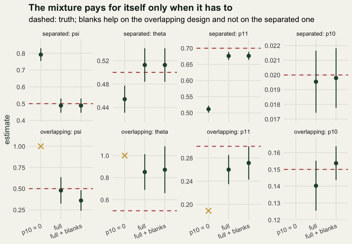
Scoring the replicate-count rule
Most field protocols never fit a mixture. They apply a rule: call the sample positive if at least so many of its replicates amplify, then feed the calls to an ordinary occupancy model. That rule can be scored exactly. For a given threshold the per-sample false positive and false negative rates are binomial tail probabilities, and the large-sample value of the naive occupancy estimate follows from fitting the clean two-level model to the exact distribution of thresholded calls.
thr_score <- function(psi, theta, p11, p10, thr) {
  fp <- 1 - pbinom(thr - 1, n_rep, p10)
  fn <- pbinom(thr - 1, n_rep, p11)
  q1 <- theta * (1 - fn) + (1 - theta) * fp
  kk <- 0:n_samp
  pk <- psi * dbinom(kk, n_samp, q1) + (1 - psi) * dbinom(kk, n_samp, fp)
  obj <- function(par) {
    ps <- plogis(par[1])
    dd <- plogis(par[2])
    -sum(pk * log(ps * dbinom(kk, n_samp, dd) + (1 - ps) * (kk == 0)))
  }
  fit <- optim(c(0, 0), obj, method = "BFGS", hessian = TRUE)
  ps <- plogis(fit$par[1])
  se <- sqrt(solve(n_site * fit$hessian)[1, 1]) * ps * (1 - ps)
  c(fp = fp, fn = fn, psi_hat = ps, bias = ps - psi, se = se,
    rmse = sqrt((ps - psi)^2 + se^2))
}

thr_grid <- expand.grid(threshold = 1:4, p10 = c(0.02, 0.15), psi = c(0.5, 0.2))
thr_tab <- cbind(thr_grid,
                 round(t(mapply(function(a, b, cc) thr_score(cc, 0.5, 0.7, b, a),
                                thr_grid$threshold, thr_grid$p10,
                                thr_grid$psi)), 4))
print(thr_tab, row.names = FALSE)
threshold p10 psi fp fn psi_hat bias se rmse
1 0.02 0.5 0.1492 0.0001 0.8129 0.3129 0.0374 0.3151
2 0.02 0.5 0.0103 0.0013 0.5294 0.0294 0.0427 0.0518
3 0.02 0.5 0.0004 0.0113 0.5012 0.0012 0.0425 0.0425
4 0.02 0.5 0.0000 0.0580 0.5000 0.0000 0.0430 0.0430
1 0.15 0.5 0.7275 0.0001 0.9988 0.4988 0.0030 0.4988
2 0.15 0.5 0.3428 0.0013 0.9592 0.4592 0.0209 0.4597
3 0.15 0.5 0.1052 0.0113 0.7457 0.2457 0.0406 0.2491
4 0.15 0.5 0.0214 0.0580 0.5611 0.0611 0.0436 0.0751
1 0.02 0.2 0.1492 0.0001 0.7618 0.5618 0.0535 0.5644
2 0.02 0.2 0.0103 0.0013 0.2482 0.0482 0.0370 0.0608
3 0.02 0.2 0.0004 0.0113 0.2019 0.0019 0.0336 0.0337
4 0.02 0.2 0.0000 0.0580 0.2000 0.0000 0.0337 0.0337
1 0.15 0.2 0.7275 0.0001 0.9990 0.7990 0.0031 0.7990
2 0.15 0.2 0.3428 0.0013 0.9614 0.7614 0.0285 0.7620
3 0.15 0.2 0.1052 0.0113 0.6464 0.4464 0.0554 0.4498
4 0.15 0.2 0.0214 0.0580 0.3036 0.1036 0.0416 0.1116for (ps in c(0.5, 0.2)) {
for (pp in c(0.02, 0.15)) {
s <- thr_tab[thr_tab$psi == ps & thr_tab$p10 == pp, ]
cat("occupancy", ps, "contamination", pp, "best threshold by rmse:",
s$threshold[which.min(s$rmse)], "\n")
}
}occupancy 0.5 contamination 0.02 best threshold by rmse: 3
occupancy 0.5 contamination 0.15 best threshold by rmse: 4
occupancy 0.2 contamination 0.02 best threshold by rmse: 3
occupancy 0.2 contamination 0.15 best threshold by rmse: 4 cat("false negative rate per sample when p11 is only",
truth_b[3], ":", round(pbinom(0:3, n_rep, truth_b[3]), 4), "\n")false negative rate per sample when p11 is only 0.3 : 0.0576 0.2553 0.5518 0.8059 At a contamination rate of 0.02 the rule works and the familiar setting is close to right. Requiring at least two of eight replicates cuts the per-sample false positive rate from 0.1492 to 0.0103 while raising the false negative rate only from 0.0001 to 0.0013, and the residual bias in occupancy falls from 0.3129 to 0.0294. Requiring three removes it (bias 0.0012) at a false negative cost of 0.0113.
At a contamination rate of 0.15 no member of the family is usable. Three of eight still leaves the occupancy estimate at 0.7457 against a truth of 0.5, and even four of eight leaves 0.5611. When the species is rarer the same rates do more damage: at a true occupancy of 0.2, three of eight gives 0.6464 and four of eight 0.3036, because the false positives are drawn from a larger pool of empty sites.
The last line of output is the other side of the trade. With p11 at 0.3 rather than 0.7, requiring four of eight replicates would discard 0.8059 of the samples that genuinely contain DNA. So the best threshold moves with p10, and how much the residual bias hurts moves with psi, and neither is known before the survey. A threshold is a defensible summary only when the two components are far apart, which is exactly the case in which the mixture model was cheap anyway.
pan_txt <- paste0("occupancy ", thr_tab$psi, ", contamination ", thr_tab$p10)
thr_long <- do.call(rbind, lapply(c("bias", "se"), function(q) {
  data.frame(threshold = thr_tab$threshold, panel = pan_txt,
             quantity = unname(c(bias = "bias",
                                 se = "standard error")[q]),
             value = thr_tab[[q]])
}))
thr_long$panel <- factor(thr_long$panel,
                         levels = unique(pan_txt[order(-thr_tab$psi,
                                                       thr_tab$p10)]))

ggplot(thr_long, aes(threshold, value, colour = quantity)) +
  geom_line(linewidth = 1) +
  geom_point(size = 2.2) +
  facet_wrap(~panel, scales = "free_y") +
  scale_colour_manual(values = c(bias = te_pal$clay,
                                 `standard error` = te_pal$forest),
                      name = NULL) +
  labs(title = "A threshold cannot be chosen without knowing p10",
       subtitle = "naive occupancy estimator applied to thresholded calls, eight replicates per sample",
       x = "positive replicates required to call a sample positive",
       y = "value") +
  theme_te()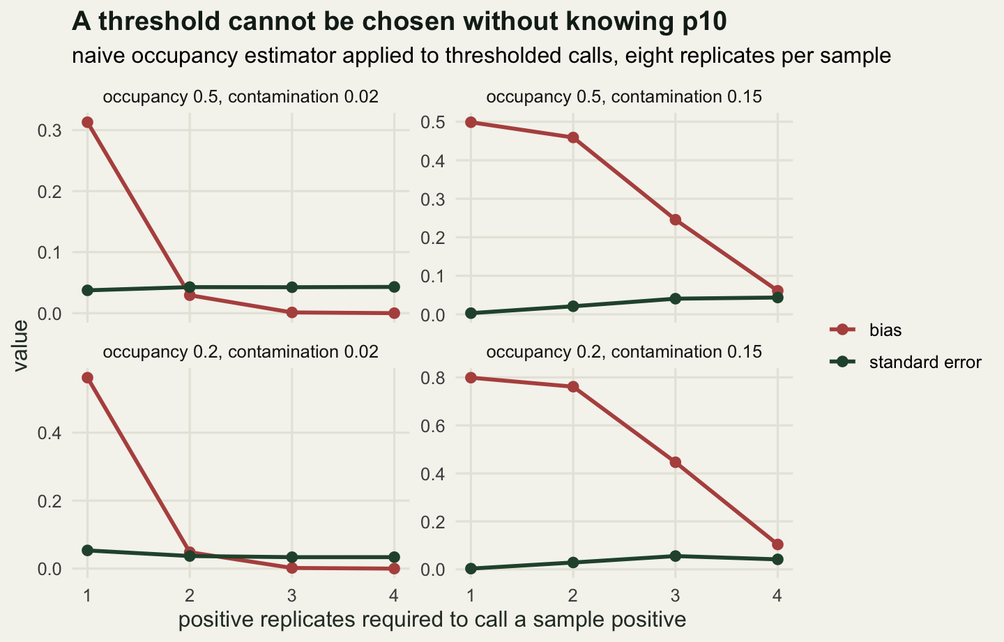
What the survey cannot tell you
Nothing above separates contamination from genuine rare DNA using survey data alone. The mixture worked on the separated design because the two components produce differently shaped replicate counts, not because the model can inspect a tube. When the shapes converge the likelihood becomes close to indifferent, and the correlation of -0.6794 is what that looks like in output. The identifying information has to come from blanks or from sites whose status is known independently, which makes negative controls part of the design rather than a courtesy to reviewers.
The constraint that p11 exceeds p10 is also load-bearing. Without it the likelihood has a mirror solution in which the labels are exchanged, and the fit is equally good. Imposing the ordering removes the ambiguity but does not test it: if a run really were more likely to produce a positive from clean water than from a DNA-bearing sample, the constraint would quietly report the inverted answer as though it were fine, and no diagnostic in the output would object.
The assumption most likely to fail in practice is independence. The mixture treats replicates as independent accidents given the sample. Real contamination arrives in clumps: one dirty plate, one net moved between ponds without bleach, one tag-jumping sequencing run. Clumped contamination inflates several replicates of the same sample together, so it mimics real DNA rather than noise, and the model cannot see the difference. Only the design catches it. Put blanks at every level, one field blank per site, one extraction blank per batch, one PCR negative per plate, and randomise samples across plates so a plate effect cannot line up with a site, a date or a treatment group. A positive blank then says where the problem entered, which is more than any likelihood recovers afterwards.
Where to go next
The measurements here turn into a design question. Replicates buy separation between the two components as well as detection probability, blanks buy identifiability only when that separation is poor, and both compete with sites for the same budget. The next tutorial spends a fixed number of PCR reactions across sites, samples and replicates and works out which allocation gives the smallest error in occupancy.
References
Royle JA, Link WA 2006 Ecology 87(4):835-841 (10.1890/0012-9658(2006)87[835:GSOMAF]2.0.CO;2)
Miller DA, Nichols JD, McClintock BT, Grant EHC, Bailey LL, Weir LA 2011 Ecology 92(7):1422-1428 (10.1890/10-1396.1)
Lahoz-Monfort JJ, Guillera-Arroita G, Tingley R 2016 Molecular Ecology Resources 16(3):673-685 (10.1111/1755-0998.12486)
Guillera-Arroita G, Lahoz-Monfort JJ, van Rooyen AR, Weeks AR, Tingley R 2017 Methods in Ecology and Evolution 8(9):1081-1091 (10.1111/2041-210X.12743)
Ficetola GF, Taberlet P, Coissac E 2016 Molecular Ecology Resources 16(3):604-607 (10.1111/1755-0998.12508)