Checking an eDNA occupancy analysis

Four checks for a three-level eDNA occupancy model in R: detection heterogeneity, predictive checks, transported DNA, and pinning the contamination rate.

An eDNA survey delivers a table of PCR results, and a three-level model turns it into an occupancy estimate with a confidence interval. The three tutorials before this one built that machinery: the site, sample and replicate likelihood with psi, theta and p; contamination as a replicate-level mixture; and how to spend a budget across the three levels. This one asks what would have to be true for the output to mean anything, on simulated surveys where the answer is known.

Four checks. Is detection really constant across samples, does a predictive check on the count distribution notice when it is not, what happens when DNA arrives at a site the animal never visited, and how much data it takes to estimate a contamination rate at all.

library(ggplot2)

te_pal <- list(forest = "#275139", green = "#2f8f63", sage = "#93a87f",
               clay = "#b5534e", gold = "#cda23f", line = "#dad9ca",
               ink = "#16241d", paper = "#f5f4ee")

theme_te <- function() {
  theme_minimal(base_size = 12) +
    theme(panel.grid.minor = element_blank(),
          panel.grid.major = element_line(colour = "#e7e6dc"),
          plot.background = element_rect(fill = "#f5f4ee", colour = NA),
          panel.background = element_rect(fill = "#f5f4ee", colour = NA),
          plot.title = element_text(face = "bold", colour = te_pal$ink),
          axis.title = element_text(colour = "#2c3a31"))
}

The likelihood in one function

A site is occupied with probability psi. Each water sample from an occupied site captures DNA with probability theta. Each PCR replicate of a DNA-bearing sample turns positive with probability p11, and each replicate of a DNA-free sample with probability p10, the contamination rate. The count of positive replicates per sample is all the data there is, so the site-level likelihood is a two-term mixture over occupancy with a second mixture over DNA presence inside it.

sim_edna <- function(n_site, n_samp, n_rep, psi, theta, p11, p10 = 0,
                     conc = NULL, tau = 0, theta_move = 0) {
  occ <- rbinom(n_site, 1, psi)
  has_dna <- occ
  if (tau > 0) {
    arrived <- (rbinom(n_site, 1, tau) == 1) & (occ == 0)
    has_dna[arrived] <- 1
  }
  th <- ifelse(occ == 1, theta, theta_move)
  th[has_dna == 0] <- 0
  present <- matrix(rbinom(n_site * n_samp, 1, rep(th, times = n_samp)),
                    n_site, n_samp)
  pdet <- matrix(p10, n_site, n_samp)
  hit <- present == 1
  if (is.null(conc)) {
    pdet[hit] <- p11
  } else {
    pdet[hit] <- rbeta(sum(hit), p11 * conc, (1 - p11) * conc)
  }
  list(y = matrix(rbinom(n_site * n_samp, n_rep, as.vector(pdet)),
                  n_site, n_samp), occ = occ, has_dna = has_dna)
}

edna_nll <- function(par, y, n_rep, p10_fix = NULL, y_neg = NULL) {
  psi <- plogis(par[1])
  theta <- plogis(par[2])
  p11 <- plogis(par[3])
  p10 <- if (is.null(p10_fix)) plogis(par[4]) else p10_fix
  in_dna <- log(psi) + rowSums(log(theta * dbinom(y, n_rep, p11) +
                                     (1 - theta) * dbinom(y, n_rep, p10)))
  no_dna <- log1p(-psi) + rowSums(dbinom(y, n_rep, p10, log = TRUE))
  ll <- sum(pmax(in_dna, no_dna) + log1p(exp(-abs(in_dna - no_dna))))
  if (!is.null(y_neg)) ll <- ll + sum(dbinom(y_neg, n_rep, p10, log = TRUE))
  if (!is.finite(ll)) return(1e10)
  -ll
}

fit_edna <- function(y, n_rep, p10_fix = 0, y_neg = NULL) {
  o <- optim(c(0, 0, 0), edna_nll, y = y, n_rep = n_rep, p10_fix = p10_fix,
             y_neg = y_neg, method = "BFGS")
  c(psi = plogis(o$par[1]), theta = plogis(o$par[2]),
    p11 = plogis(o$par[3]), nll = o$value)
}

The mixture branches are combined on the log scale with the shifted log-sum-exp identity rather than by exponentiating, which keeps the fit stable when a site contributes a very small probability. The argument y_neg takes counts from samples known to hold no target DNA: lab blanks, which enter the likelihood through p10 alone, used in Check 4.

The optional arguments of sim_edna are the three ways the truth will be made to differ from the model: conc gives every sample its own detection probability, p10 adds contamination, and tau with theta_move lets DNA arrive at unoccupied sites.

Check 1: is detection constant across samples?

The model assigns one p11 to every DNA-bearing sample, while real samples differ in DNA concentration, inhibitor load and filter volume. Simulate a survey where the per-sample detection probability is drawn from a beta distribution with the same mean as the homogeneous case, fit the homogeneous model to both, and compare.

n_site <- 120
n_samp <- 5
n_rep <- 6
psi_true <- 0.55
theta_true <- 0.60
p_true <- 0.45

set.seed(20260812)
dat_hom <- sim_edna(n_site, n_samp, n_rep, psi_true, theta_true, p_true)
dat_het <- sim_edna(n_site, n_samp, n_rep, psi_true, theta_true, p_true,
                    conc = 2)
fit_hom <- fit_edna(dat_hom$y, n_rep)
fit_het <- fit_edna(dat_het$y, n_rep)

cat("sites", n_site, "samples per site", n_samp,
    "replicates per sample", n_rep, "\n")

sites 120 samples per site 5 replicates per sample 6 

cat("sites with at least one positive replicate: homogeneous",
    sum(rowSums(dat_hom$y) > 0), " heterogeneous",
    sum(rowSums(dat_het$y) > 0), "\n")

sites with at least one positive replicate: homogeneous 69  heterogeneous 68 

est_tab <- data.frame(
  source = c("truth", "fit to homogeneous", "fit to heterogeneous"),
  psi = round(c(psi_true, fit_hom["psi"], fit_het["psi"]), 4),
  theta = round(c(theta_true, fit_hom["theta"], fit_het["theta"]), 4),
  p = round(c(p_true, fit_hom["p11"], fit_het["p11"]), 4))
print(est_tab, row.names = FALSE)

               source    psi  theta      p
                truth 0.5500 0.6000 0.4500
   fit to homogeneous 0.5848 0.5751 0.4469
 fit to heterogeneous 0.5939 0.4667 0.5101

One survey cannot separate bias from sampling noise, so repeat both truths sixty times and average.

n_run <- 60
runs <- matrix(NA_real_, n_run, 6)
for (r in seq_len(n_run)) {
  a <- sim_edna(n_site, n_samp, n_rep, psi_true, theta_true, p_true)
  b <- sim_edna(n_site, n_samp, n_rep, psi_true, theta_true, p_true, conc = 2)
  runs[r, 1:3] <- fit_edna(a$y, n_rep)[1:3]
  runs[r, 4:6] <- fit_edna(b$y, n_rep)[1:3]
}
bias_tab <- data.frame(
  parameter = c("psi", "theta", "p"),
  truth = c(psi_true, theta_true, p_true),
  mean_homogeneous = round(colMeans(runs)[1:3], 4),
  mean_heterogeneous = round(colMeans(runs)[4:6], 4))
bias_tab$bias <- round(bias_tab$mean_heterogeneous - bias_tab$truth, 4)
cat("replicate data sets per truth:", n_run, "\n")

replicate data sets per truth: 60 

print(bias_tab, row.names = FALSE)

 parameter truth mean_homogeneous mean_heterogeneous    bias
       psi  0.55           0.5428             0.5516  0.0016
     theta  0.60           0.6072             0.4978 -0.1022
         p  0.45           0.4491             0.5455  0.0955

The bias goes somewhere specific. Occupancy is almost untouched: psi averages 0.5516 against a true 0.55, a bias of 0.0016, which is smaller than the noise. The two lower-level parameters absorb the whole misfit, in opposite directions. Sample-level capture falls from 0.6 to 0.4978, a bias of -0.1022, and replicate-level detection rises from 0.45 to 0.5455, a bias of 0.0955.

The mechanism is visible once you ask where a low-p11 sample goes. A sample with an unlucky draw yields zero positives out of six replicates, which the homogeneous model cannot tell apart from a sample that never held DNA, so it is booked as DNA-free and theta drops. What remains among the positive samples is enriched for high-p11 draws, so p11 rises. Occupancy survives because it depends mainly on how many sites produced any positive at all, and that count barely moves: 69 sites under homogeneous detection and 68 under heterogeneous.

That is the good news and the trap. A paper reporting only psi would be fine here; a paper reporting theta and p11 as design guidance, saying how many samples and replicates the next survey needs, would be wrong in both directions at once.

The check that catches it without knowing the truth uses the shape of the count distribution. Among samples with at least one positive, the number of positives should follow a binomial with p11, truncated below at one. Heterogeneous detection adds mass at both ends and inflates the variance.

count_check <- function(y, p, n_rep) {
  v <- as.vector(y)
  v <- v[v > 0]
  pr <- dbinom(1:n_rep, n_rep, p) / (1 - dbinom(0, n_rep, p))
  fitted_var <- sum((1:n_rep)^2 * pr) - sum((1:n_rep) * pr)^2
  expected <- length(v) * pr
  observed <- tabulate(v, n_rep)
  list(stat = c(positive_samples = length(v), obs_var = var(v),
                fitted_var = fitted_var, ratio = var(v) / fitted_var,
                chisq = sum((observed - expected)^2 / expected)),
       observed = observed, expected = expected)
}
cc_hom <- count_check(dat_hom$y, fit_hom["p11"], n_rep)
cc_het <- count_check(dat_het$y, fit_het["p11"], n_rep)
print(round(rbind(homogeneous = cc_hom$stat, heterogeneous = cc_het$stat), 4))

              positive_samples obs_var fitted_var  ratio    chisq
homogeneous                196  1.2499     1.3086 0.9552   1.6628
heterogeneous              164  2.7315     1.3873 1.9690 129.9449

shape_tab <- data.frame(
  positives = 1:n_rep,
  obs_hom = cc_hom$observed, exp_hom = round(cc_hom$expected, 1),
  obs_het = cc_het$observed, exp_het = round(cc_het$expected, 1))
print(shape_tab, row.names = FALSE)

 positives obs_hom exp_hom obs_het exp_het
         1      29    28.0      38    14.4
         2      51    56.6      28    37.4
         3      66    60.9      32    51.9
         4      39    36.9      29    40.5
         5      10    11.9      19    16.9
         6       1     1.6      18     2.9

cat("chi-squared five percent point on four degrees of freedom:",
    round(qchisq(0.95, 4), 2), "\n")

chi-squared five percent point on four degrees of freedom: 9.49 

The check fires only where it should. On homogeneous data the observed variance among positive samples is 1.2499 against a fitted 1.3086, a ratio of 0.9552, and the discrepancy statistic is 1.6628. On heterogeneous data the variance is 2.7315 against 1.3873, a ratio of 1.969, and the statistic is 129.9449 against a five percent point of 9.49 on four degrees of freedom.

The cell that does the damage is the top one. Eighteen samples went six for six where the fitted model expects 2.9, and 38 went one for six against an expected 14.4. Both tails at once is the signature of variable detection; one tail alone is not, since too many all-positive samples would simply mean p11 is higher than fitted.

count_df <- rbind(
  data.frame(positives = 1:n_rep, observed = cc_hom$observed,
             fitted = cc_hom$expected, truth = "detection constant"),
  data.frame(positives = 1:n_rep, observed = cc_het$observed,
             fitted = cc_het$expected, truth = "detection varies by sample"))

ggplot(count_df, aes(positives, observed)) +
  geom_col(fill = te_pal$sage, colour = "white", width = 0.75) +
  geom_point(aes(y = fitted), colour = te_pal$clay, size = 2.6) +
  geom_line(aes(y = fitted), colour = te_pal$clay, linewidth = 0.6) +
  facet_wrap(~truth) +
  scale_x_continuous(breaks = 1:n_rep) +
  labs(title = "Where variable detection shows up",
       subtitle = "bars: observed samples; points: expectation under the fitted model",
       x = "positive replicates in the sample", y = "samples") +
  theme_te()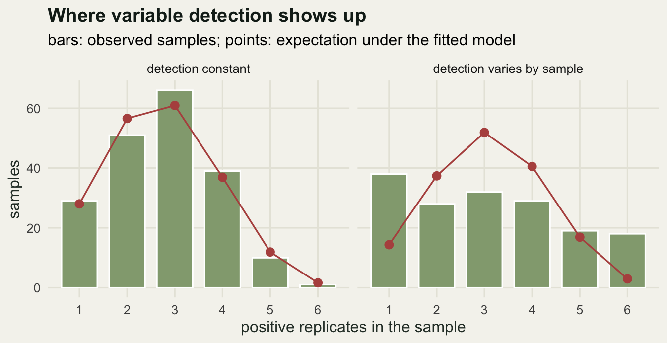

Figure 1: Observed and fitted distribution of positive replicates among samples with at least one positive, under homogeneous and heterogeneous replicate detection.

Check 2: a predictive check is only as good as its summary

The statistic above was chosen because it targets the failure. A general purpose check has no such advantage, and it is worth seeing what the choice of summary costs. Fit the model, simulate many surveys from the fitted parameters, and compare an observed summary against its predictive distribution. Use one summary the likelihood already matches and one it does not.

post_summaries <- function(y) c(total = sum(y), singletons = sum(y == 1))
n_boot_main <- 500
predictive <- function(fit, y_obs, n_boot = n_boot_main) {
  obs <- post_summaries(y_obs)
  sims <- t(replicate(n_boot, post_summaries(
    sim_edna(n_site, n_samp, n_rep, fit["psi"], fit["theta"],
             fit["p11"])$y)))
  list(obs = obs, sims = sims,
       p = (1 + colSums(sims >= rep(obs, each = n_boot))) / (n_boot + 1))
}
cat("predictive data sets simulated per check:", n_boot_main, "\n")

predictive data sets simulated per check: 500 

pc_hom <- predictive(fit_hom, dat_hom$y)
pc_het <- predictive(fit_het, dat_het$y)
ppc_tab <- data.frame(
  data_set = c("homogeneous", "homogeneous", "heterogeneous", "heterogeneous"),
  summary_used = rep(c("positive replicates", "single-positive samples"), 2),
  observed = c(pc_hom$obs, pc_het$obs),
  predicted_mean = round(c(colMeans(pc_hom$sims), colMeans(pc_het$sims)), 1),
  p_value = round(c(pc_hom$p, pc_het$p), 4))
print(ppc_tab, row.names = FALSE)

      data_set            summary_used observed predicted_mean p_value
   homogeneous     positive replicates      541          540.0  0.4731
   homogeneous single-positive samples       29           27.8  0.4531
 heterogeneous     positive replicates      509          508.7  0.5090
 heterogeneous single-positive samples       38           14.4  0.0020

The total number of positive replicates cannot fail. On the heterogeneous survey the observed total is 509 against a predictive mean of 508.7, p-value 0.509, and on the homogeneous survey 541 against 540.0, p-value 0.4731. Fitting theta and p11 is what sets how much positive signal the model expects, so the fit reproduces that total almost exactly and the check is close to empty no matter how wrong the model is.

Counting samples with exactly one positive replicate is a different matter. On the homogeneous survey it gives 29 observed against 27.8 predicted, p-value 0.4531, and on the heterogeneous survey 38 against 14.4, with a p-value of 0.002, the smallest the 500 simulations can express.

So a predictive check is not a property of the model. It is a property of the summary, and a summary in the span of the fitted moments has no power at all. Choose summaries the likelihood does not control: counts in single cells of the replicate distribution, the spread among sites, the number of sites resting on one positive sample.

mk <- function(pc, nm) rbind(
  data.frame(value = pc$sims[, 1], obs = as.numeric(pc$obs[1]),
             panel = paste(nm, "positive replicates", sep = ": ")),
  data.frame(value = pc$sims[, 2], obs = as.numeric(pc$obs[2]),
             panel = paste(nm, "single-positive samples", sep = ": ")))
ppc_df <- rbind(mk(pc_hom, "detection constant"),
                mk(pc_het, "detection varies"))

ggplot(ppc_df, aes(value)) +
  geom_histogram(bins = 24, fill = te_pal$sage, colour = "white") +
  geom_vline(aes(xintercept = obs), colour = te_pal$clay, linewidth = 0.9) +
  facet_wrap(~panel, scales = "free", ncol = 2) +
  labs(title = "The summary decides whether the check can fail",
       subtitle = "red line: observed value; histogram: simulations from the fitted model",
       x = "summary value", y = "simulated surveys") +
  theme_te()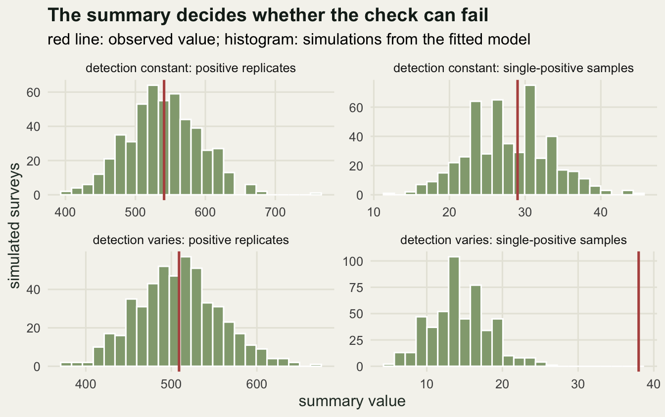

Figure 2: Predictive distributions of two summaries under the fitted model, with the observed value marked, for the homogeneous and heterogeneous surveys.

Check 3: the assumption no internal check can reach

DNA moves. It washes downstream, it rides on boots and boats, it sits in sediment after the animal has gone. A DNA-positive site is therefore not the same object as an occupied site, and no rearrangement of the likelihood can separate them, because the data hold no variable that distinguishes local production from arrival.

Simulate that. A fraction tau of the unoccupied sites receives transported DNA at a reduced concentration, so their sample-level capture probability is 0.15 rather than 0.6, and fit the standard model.

taus <- c(0, 0.1, 0.2, 0.3, 0.4, 0.5)
theta_move <- 0.15
n_move_run <- 12
n_boot_sweep <- 300
cat("theta at a transport-only site:", theta_move,
    " data sets per transport rate:", n_move_run,
    " predictive data sets:", n_boot_sweep, "\n")

theta at a transport-only site: 0.15  data sets per transport rate: 12  predictive data sets: 300 

move_tab <- NULL
for (tt in taus) {
  psis <- numeric(n_move_run)
  pv <- c(NA, NA)
  for (r in seq_len(n_move_run)) {
    d <- sim_edna(n_site, n_samp, n_rep, psi_true, theta_true, p_true,
                  tau = tt, theta_move = theta_move)
    fq <- fit_edna(d$y, n_rep)
    psis[r] <- fq["psi"]
    if (r == 1) pv <- predictive(fq, d$y, n_boot = n_boot_sweep)$p
  }
  move_tab <- rbind(move_tab, data.frame(
    tau = tt,
    dna_occupancy = psi_true + tt * (1 - psi_true),
    psi_hat = round(mean(psis), 4),
    p_total = round(pv[1], 3),
    p_singletons = round(pv[2], 3)))
}
print(move_tab, row.names = FALSE)

 tau dna_occupancy psi_hat p_total p_singletons
 0.0         0.550  0.5452   0.508        0.864
 0.1         0.595  0.5847   0.485        0.615
 0.2         0.640  0.5948   0.475        0.409
 0.3         0.685  0.6443   0.532        0.801
 0.4         0.730  0.6360   0.535        0.259
 0.5         0.775  0.6944   0.455        0.116

cat("inflation of psi at the highest transport rate:",
    round(move_tab$psi_hat[nrow(move_tab)] - psi_true, 4), "\n")

inflation of psi at the highest transport rate: 0.1444 

cat("smallest predictive p-value over the sweep:",
    round(min(c(move_tab$p_total, move_tab$p_singletons)), 3), "\n")

smallest predictive p-value over the sweep: 0.116 

The estimate climbs from 0.5452 with no transport to 0.6944 when half the empty sites receive DNA, an inflation of 0.1444 on a true organism occupancy of 0.55. Nor does it reach the DNA occupancy of 0.775, because transported sites carry weak signal and many stay entirely negative. What the model reports has no clean definition: somewhere between the occupancy of the animal and the occupancy of its DNA, with the mixture set by a transport rate the data cannot see.

Meanwhile the diagnostics stay silent. The smallest predictive p-value anywhere in the sweep is 0.116, because transport changes how many sites hold DNA, not the shape of the replicate distribution inside a DNA-bearing sample. The model is not misfitting. It is fitting a different quantity than the one the paper title claims, and misfit tests cannot see a definitional error.

What does catch it is design, built in before sampling. Paired upstream and downstream samples at the same site turn transport into a testable gradient, because production is local and transport is directional. A second detection method at a subset of sites, trapping or a visual survey, gives an external occupancy estimate that the eDNA one can be calibrated against. And a concentration threshold set against samples from known presences discards the weak positives that transport mostly produces, at the price of a lower theta the model can absorb honestly.

move_df <- rbind(
  data.frame(tau = move_tab$tau, value = move_tab$psi_hat,
             series = "estimated psi"),
  data.frame(tau = move_tab$tau, value = move_tab$dna_occupancy,
             series = "true DNA occupancy"),
  data.frame(tau = move_tab$tau, value = psi_true,
             series = "true organism occupancy"))

ggplot(move_df, aes(tau, value, colour = series, linetype = series)) +
  geom_line(linewidth = 0.9) +
  geom_point(size = 2.2) +
  scale_colour_manual(values = c(`estimated psi` = te_pal$clay,
                                 `true DNA occupancy` = te_pal$gold,
                                 `true organism occupancy` = te_pal$forest),
                      name = NULL) +
  scale_linetype_manual(values = c(`estimated psi` = "solid",
                                   `true DNA occupancy` = "dashed",
                                   `true organism occupancy` = "dotted"),
                        name = NULL) +
  labs(title = "Transported DNA inflates occupancy",
       subtitle = "the model estimates neither the animal nor its DNA",
       x = "fraction of unoccupied sites receiving DNA",
       y = "occupancy") +
  theme_te() +
  theme(legend.position = "bottom")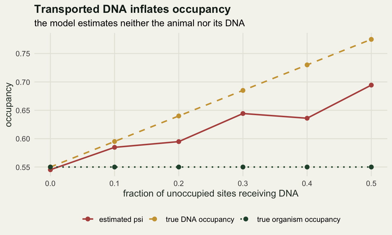

Figure 3: Estimated occupancy against the fraction of unoccupied sites receiving transported DNA, with the true organism occupancy and the true DNA occupancy for comparison.

Check 4: how much data identifies the contamination rate?

Turning p10 loose is the standard answer to false positives, and it is worth knowing what the data say about it before trusting the result. Profile the likelihood over p10 with psi, theta and p11 free at each grid point, on surveys of increasing size, and read off the interval where the profile stays within two log-likelihood units of its maximum.

p10_true <- 0.005
p10_grid <- seq(2e-4, 0.03, length.out = 60)
prof_p10 <- function(y, y_neg = NULL) {
  z <- sapply(p10_grid, function(q) {
    fq <- fit_edna(y, n_rep, p10_fix = q, y_neg = y_neg)
    c(-fq["nll"], fq["psi"])
  })
  data.frame(p10 = p10_grid, loglik = z[1, ], psi = z[2, ])
}
span_two <- function(pf) {
  keep <- (pf$loglik - max(pf$loglik)) >= -2
  c(mle = pf$p10[which.max(pf$loglik)],
    lower = min(pf$p10[keep]), upper = max(pf$p10[keep]),
    width = max(pf$p10[keep]) - min(pf$p10[keep]),
    psi_lower = min(pf$psi[keep]), psi_upper = max(pf$psi[keep]))
}

d_small <- sim_edna(40, n_samp, n_rep, psi_true, theta_true, p_true,
                    p10 = p10_true)
d_mid <- sim_edna(160, n_samp, n_rep, psi_true, theta_true, p_true,
                  p10 = p10_true)
d_big <- sim_edna(640, n_samp, n_rep, psi_true, theta_true, p_true,
                  p10 = p10_true)
psi_common <- 0.90
d_common <- sim_edna(160, n_samp, n_rep, psi_common, theta_true, p_true,
                     p10 = p10_true)
n_blank <- 200
y_blank <- rbinom(n_blank, n_rep, p10_true)

prof_list <- list(prof_p10(d_small$y), prof_p10(d_mid$y), prof_p10(d_big$y),
                  prof_p10(d_common$y), prof_p10(d_common$y, y_blank))
prof_lab <- c("40 sites", "160 sites", "640 sites",
              "160 sites, psi 0.9", "160 sites, psi 0.9, 200 blanks")
prof_tab <- data.frame(design = prof_lab,
                       round(do.call(rbind, lapply(prof_list, span_two)), 4))
print(prof_tab, row.names = FALSE)

                         design    mle  lower  upper  width psi_lower psi_upper
                       40 sites 0.0032 0.0002 0.0103 0.0101    0.5540    0.6280
                      160 sites 0.0063 0.0032 0.0108 0.0076    0.5941    0.6083
                      640 sites 0.0037 0.0027 0.0053 0.0025    0.5544    0.5604
             160 sites, psi 0.9 0.0017 0.0002 0.0103 0.0101    0.9331    0.9432
 160 sites, psi 0.9, 200 blanks 0.0037 0.0017 0.0073 0.0056    0.9343    0.9397

cat("true false-positive rate:", p10_true,
    " occupancy in the common-species design:", psi_common, "\n")

true false-positive rate: 0.005  occupancy in the common-species design: 0.9 

cat("unoccupied sites available as internal blanks: 40 ->",
    sum(d_small$occ == 0), " 160 ->", sum(d_mid$occ == 0), " 640 ->",
    sum(d_big$occ == 0), " common ->", sum(d_common$occ == 0), "\n")

unoccupied sites available as internal blanks: 40 -> 18  160 -> 62  640 -> 286  common -> 11 

cat("positive replicates among the", n_blank, "known blanks:", sum(y_blank),
    "of", n_blank * n_rep, "\n")

positive replicates among the 200 known blanks: 5 of 1200 

cat("width reduction from the blanks, percent:",
    round(100 * (1 - prof_tab$width[5] / prof_tab$width[4]), 1), "\n")

width reduction from the blanks, percent: 44.6 

cat("span of psi across the two-unit interval: 40 sites",
    round(prof_tab$psi_upper[1] - prof_tab$psi_lower[1], 4), " 640 sites",
    round(prof_tab$psi_upper[3] - prof_tab$psi_lower[3], 4), "\n")

span of psi across the two-unit interval: 40 sites 0.074  640 sites 0.006 

At 40 sites the interval runs from the grid floor of 0.0002 up to 0.0103, a width of 0.0101 around a true rate of 0.005. It includes zero for practical purposes, so the survey cannot separate a clean lab from a contamination rate twice the truth. Psi moves by 0.074 across that interval, which is the number that matters: the occupancy estimate is only as sharp as the contamination rate it assumes.

The narrowing is slow. The width is 0.0076 at 160 sites and 0.0025 at 640, where the interval runs from 0.0027 to 0.0053 and psi spans only 0.006. So p10 becomes usable somewhere between 160 and 640 sites here, four to sixteen times the size of a typical single-catchment survey.

The reason is easy to miss and it changes the design advice. Information about p10 comes almost entirely from sites where the species is absent, which act as unplanned blanks: 18 at 40 sites, 62 at 160, and 286 at 640. Raise occupancy to 0.9 and they disappear. The fourth row shows it: 160 sites of a common species leave 11 empty sites, and the width goes back to 0.0101, no better than a survey a quarter of the size.

That is where lab blanks earn their cost. Adding 200 known-negative samples, which produced 5 positive replicates out of 1200, cuts the width for the common species by 44.6 percent. Negative controls are usually treated as a quality-assurance step, something you inspect and hope is empty. In this model they are data, they enter the likelihood directly, and they are the only source of information about p10 that does not need the species to be rare.

panel_lev <- c("survey size, occupancy 0.55", "common species, 160 sites")
prof_df <- do.call(rbind, lapply(seq_along(prof_list), function(k) {
  pf <- prof_list[[k]]
  data.frame(p10 = pf$p10, rel = pf$loglik - max(pf$loglik),
             design = prof_lab[k],
             panel = if (k <= 3) panel_lev[1] else panel_lev[2])
}))
prof_df$design <- factor(prof_df$design, levels = prof_lab)
prof_df$panel <- factor(prof_df$panel, levels = panel_lev)

ggplot(prof_df, aes(p10, rel, colour = design)) +
  geom_hline(yintercept = -2, colour = te_pal$ink, linetype = "dashed",
             linewidth = 0.5) +
  geom_vline(xintercept = p10_true, colour = te_pal$ink, linetype = "dotted",
             linewidth = 0.5) +
  geom_line(linewidth = 1) +
  facet_wrap(~panel) +
  coord_cartesian(ylim = c(-8, 0.4)) +
  scale_colour_manual(values = c(te_pal$sage, te_pal$green, te_pal$forest,
                                 te_pal$gold, te_pal$clay), name = NULL) +
  labs(title = "How sharply is the contamination rate pinned?",
       subtitle = "dotted vertical: the true rate; dashed horizontal: two log-likelihood units down",
       x = "false-positive rate per replicate",
       y = "profile log-likelihood minus its maximum") +
  theme_te() +
  theme(legend.position = "bottom") +
  guides(colour = guide_legend(nrow = 2))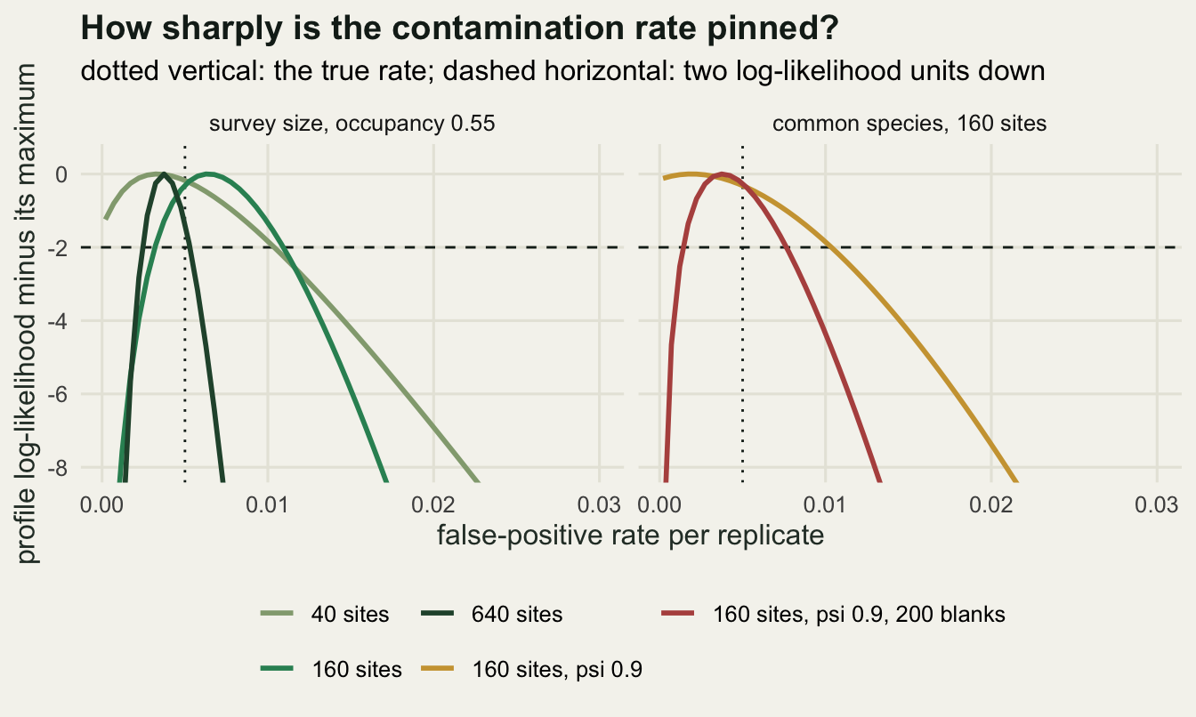

Figure 4: Profile log-likelihood for the false-positive rate, by survey size at moderate occupancy and for a common species with and without known-negative samples.

What the four checks leave standing

The four checks constrain the analysis; none of them validates it. Two failures pass all of them.

The first is DNA that did not come from a living local individual. Check 3 measured one version, transport, and the others are worse because they are less regular: a dead animal, a predator’s gut contents deposited far from any population, sediment DNA resuspended from a decade ago. Each produces a genuine positive at a site the species does not occupy, the likelihood has no term for any of them, and the predictive checks stay clean because nothing about the count distribution is odd.

The second is contamination that is correlated rather than independent. The p10 term treats each replicate as an independent coin flip, which is the wrong picture for a bad plate, a net moved between sites without disinfection, or field blanks opened in the same tent as the samples. Correlated false positives arrive in clusters that look exactly like true detections: several positives in one sample, several samples at one site. That is the pattern the model was built to read as occupancy, so it will, and a wider interval on p10 does not help because the failure is in the independence assumption rather than in the rate.

Both are design problems, and the honest fix is a protocol rather than a better likelihood: controls at every level, field blanks handled apart from the samples, randomised plate layouts, and an independent detection method at a subset of sites to anchor what the eDNA estimate is estimating. The likelihood is still worth building, because it makes the assumptions explicit and because Check 1 and Check 2 do catch real failures. It is not worth trusting on its own.

Where to go next

The general version of this argument sits in the occupancy cluster, where the tutorial on checking an occupancy variant applies the same logic to models with covariates and several seasons: which parts of a fitted occupancy model the data constrain, and which parts the reader takes on faith.

References

Barnes MA, Turner CR 2016 Conservation Genetics 17(1):1-17 (10.1007/s10592-015-0775-4)

Jane SF et al 2015 Molecular Ecology Resources 15(1):216-227 (10.1111/1755-0998.12285)

Goldberg CS et al 2016 Methods in Ecology and Evolution 7(11):1299-1307 (10.1111/2041-210X.12595)

Guillera-Arroita G 2017 Ecography 40(2):281-295 (10.1111/ecog.02445)

Related tutorials

• Three-level occupancy models for eDNA
• False positives in eDNA surveys
• Sampling design for eDNA surveys
• Checking an occupancy variant