Sampling design for eDNA surveys

Split an eDNA budget between sites, water samples and PCR replicates in R, with exact asymptotic precision for occupancy and a measured optimal design.

An eDNA survey has three numbers in it and one budget to cover all three: how many sites to visit, how many water samples to filter at each site, how many PCR replicates to run from each sample. They are not interchangeable. A site visit costs travel and a day, a sample costs a filter and an extraction, a replicate costs one well on a plate, and each level buys a different kind of certainty.

The two-level version of this problem is already solved in How many visits? Occupancy survey design, which is the prerequisite here: a fixed budget of site visits, exact asymptotic standard errors from the Fisher information, and an answer for how many visits a site needs. This tutorial does the three-level version with a different unit cost at each level, computes the precision every affordable design delivers, and then spends the money.

The likelihood, rebuilt

A site is occupied with probability psi. Inside an occupied site, each water sample carries detectable DNA with probability theta. Inside such a sample, each PCR replicate comes up positive with probability p. Nothing else is ever positive, so this post assumes the contamination problem away and works with a clean assay.

The data from one site are the positive-replicate counts, one count per sample, each between zero and K. The distribution of a single count under occupancy is a zero-inflated binomial: with probability theta the sample holds DNA and the count is binomial, otherwise the count is zero for certain.

library(ggplot2)

te_pal <- list(forest = "#275139", green = "#2f8f63", sage = "#93a87f",
               clay = "#b5534e", gold = "#cda23f", line = "#dad9ca",
               ink = "#16241d", paper = "#f5f4ee")

theme_te <- function() {
  theme_minimal(base_size = 12) +
    theme(panel.grid.minor = element_blank(),
          panel.grid.major = element_line(colour = "#e7e6dc"),
          plot.background = element_rect(fill = "#f5f4ee", colour = NA),
          panel.background = element_rect(fill = "#f5f4ee", colour = NA),
          plot.title = element_text(face = "bold", colour = te_pal$ink),
          axis.title = element_text(colour = "#2c3a31"))
}

sample_probs <- function(theta, p, n_rep) {
  counts <- 0:n_rep
  theta * dbinom(counts, n_rep, p) + (1 - theta) * (counts == 0)
}

psi_true <- 0.4
theta_true <- 0.5
p_true <- 0.7

cat("design parameters: psi", psi_true, " theta", theta_true, " p", p_true, "\n")

design parameters: psi 0.4  theta 0.5  p 0.7 

cat("per-sample outcome probabilities at two replicates:",
    round(sample_probs(theta_true, p_true, 2), 4), "\n")

per-sample outcome probabilities at two replicates: 0.545 0.21 0.245 

cat("per-sample detection probability, one to four replicates:",
    round(theta_true * (1 - (1 - p_true)^(1:4)), 4), "\n")

per-sample detection probability, one to four replicates: 0.35 0.455 0.4865 0.496 

At two replicates a sample that holds DNA is already caught with probability 0.455 out of a ceiling of 0.5, and a third replicate raises that only to 0.4865. Those numbers are the whole argument of this post in miniature, and the rest of it is about what else the same money could have bought.

Expected information, without simulating

The asymptotic standard error of psi comes from the expected Fisher information, and for this model it can be written down rather than simulated. Given occupancy, the J samples of a site are independent draws from the outcome vector of length K + 1 computed above, so a site is a multinomial draw over K + 1 categories. The log-likelihood of any site with at least one positive replicate is linear in those category counts, which means every second moment of the score reduces to a sum over K + 1 terms instead of an enumeration of outcomes. The all-zero site is the only awkward case, because it is the one outcome that mixes the occupied and the unoccupied branch, so it gets its own term.

info_site <- function(psi, theta, p, n_samp, n_rep) {
  counts <- 0:n_rep
  bin <- dbinom(counts, n_rep, p)
  qc <- theta * bin + (1 - theta) * (counts == 0)
  dq_theta <- bin - (counts == 0)
  dq_p <- theta * bin * (counts / p - (n_rep - counts) / (1 - p))
  ratio_theta <- dq_theta / qc
  ratio_p <- dq_p / qc
  full <- matrix(0, 3, 3)
  full[1, 1] <- 1 / psi^2
  full[2, 2] <- n_samp * sum(qc * ratio_theta^2)
  full[3, 3] <- n_samp * sum(qc * ratio_p^2)
  full[2, 3] <- full[3, 2] <- n_samp * sum(qc * ratio_theta * ratio_p)
  score_zero <- c(1 / psi, n_samp * ratio_theta[1], n_samp * ratio_p[1])
  prob_zero <- psi * qc[1]^n_samp + 1 - psi
  grad_zero <- c(qc[1]^n_samp - 1,
                 psi * n_samp * qc[1]^(n_samp - 1) * dq_theta[1],
                 psi * n_samp * qc[1]^(n_samp - 1) * dq_p[1])
  psi * (full - qc[1]^n_samp * outer(score_zero, score_zero)) +
    outer(grad_zero, grad_zero) / prob_zero
}

se_psi <- function(psi, theta, p, n_sites, n_samp, n_rep) {
  info <- n_sites * info_site(psi, theta, p, n_samp, n_rep)
  if (1 / kappa(info) < 1e-10) return(NA_real_)
  sqrt(solve(info)[1, 1])
}

cat("reciprocal condition number of the information matrix\n")

reciprocal condition number of the information matrix

cat(" one sample per site:",
    format(1 / kappa(info_site(psi_true, theta_true, p_true, 1, 3)), digits = 3),
    " one replicate per sample:",
    format(1 / kappa(info_site(psi_true, theta_true, p_true, 4, 1)), digits = 3),
    "\n")

 one sample per site: 1.35e-17  one replicate per sample: 6.08e-17 

cat(" four samples, two replicates:",
    round(1 / kappa(info_site(psi_true, theta_true, p_true, 4, 2)), 4), "\n")

 four samples, two replicates: 0.3457 

Two structural facts arrive before any design work. With one sample per site the data depend on psi and theta only through their product; with one replicate per sample the same happens to theta and p. In both cases the information matrix is singular to machine precision, so no amount of budget rescues the design and the grid below starts at two samples and two replicates.

Now the check that makes the formula usable. Simulate data at a design, fit the model by maximum likelihood, and compare the spread of the estimates against what the formula promised.

sim_counts <- function(psi, theta, p, n_sites, n_samp, n_rep) {
  occupied <- rbinom(n_sites, 1, psi)
  has_dna <- rbinom(n_sites * n_samp, 1, theta * rep(occupied, n_samp))
  matrix(rbinom(n_sites * n_samp, n_rep, p * has_dna), n_sites, n_samp)
}

neg_loglik <- function(par, ymat, n_rep) {
  qc <- sample_probs(plogis(par[2]), plogis(par[3]), n_rep)
  n_samp <- ncol(ymat)
  per_site <- rowSums(matrix(log(qc)[ymat + 1], nrow(ymat), n_samp))
  found <- rowSums(ymat) > 0
  -(sum(log(plogis(par[1])) + per_site[found]) +
      sum(!found) * log(plogis(par[1]) * qc[1]^n_samp + 1 - plogis(par[1])))
}

fit_psi <- function(ymat, n_rep) {
  opt <- optim(c(0, 0, 0), neg_loglik, ymat = ymat, n_rep = n_rep,
               method = "Nelder-Mead",
               control = list(reltol = 1e-10, maxit = 800))
  c(plogis(opt$par[1]), opt$convergence)
}

set.seed(908)
n_fits <- 300
validate <- NULL
for (cfg in list(c(58, 4, 2), c(52, 4, 3))) {
  draws <- t(replicate(n_fits, fit_psi(
    sim_counts(psi_true, theta_true, p_true, cfg[1], cfg[2], cfg[3]), cfg[3])))
  validate <- rbind(validate, data.frame(
    sites = cfg[1], samples = cfg[2], replicates = cfg[3],
    mean_psi_hat = round(mean(draws[, 1]), 4),
    simulated_sd = round(sd(draws[, 1]), 4),
    asymptotic_se = round(se_psi(psi_true, theta_true, p_true,
                                 cfg[1], cfg[2], cfg[3]), 4),
    failures = sum(draws[, 2] != 0)))
}
validate$ratio <- round(validate$simulated_sd / validate$asymptotic_se, 4)
cat("maximum likelihood fits per design:", n_fits, "\n")

maximum likelihood fits per design: 300 

print(validate, row.names = FALSE)

 sites samples replicates mean_psi_hat simulated_sd asymptotic_se failures
    58       4          2       0.4117       0.0716        0.0716        0
    52       4          3       0.4092       0.0759        0.0736        0
  ratio
 1.0000
 1.0312

Three hundred maximum likelihood fits at each of two designs. At 58 sites with four samples and two replicates the formula says 0.0716 and the simulation gives 0.0716, a ratio of 1. At 52 sites with three replicates the formula says 0.0736 and the simulation gives 0.0759, a ratio of 1.0312, which is the usual small optimism of an asymptotic variance at this sample size. Both designs recover psi with a mild upward bias (0.4117 and 0.4092 against a true 0.4), also expected: the likelihood is skewed and the estimator is not unbiased in finite samples.

Spending a budget

The cost model has to be written down explicitly because everything below depends on it. A site visit costs 10, a water sample costs 4, a PCR replicate costs 1, in the same arbitrary units, and the total spend for S sites is S times the sum of the site cost and J samples each carrying its own replicates. Only the ratios matter, so substitute your own: if your sites are a boat charter apart and your plates are cheap, the site cost rises and the answer moves.

cost_site <- 10
cost_sample <- 4
cost_replicate <- 1
budget <- 2000

design_cost <- function(n_sites, n_samp, n_rep) {
  n_sites * (cost_site + n_samp * (cost_sample + n_rep * cost_replicate))
}

design_grid <- function(psi, theta, p, budget, samp_max = 10, rep_max = 9) {
  out <- NULL
  for (j in 2:samp_max) {
    for (k in 2:rep_max) {
      n_sites <- floor(budget / design_cost(1, j, k))
      if (n_sites < 2) next
      out <- rbind(out, data.frame(samples = j, replicates = k,
                                   sites = n_sites,
                                   spent = design_cost(n_sites, j, k),
                                   se = se_psi(psi, theta, p, n_sites, j, k)))
    }
  }
  out <- out[order(out$se), ]
  out$excess_pct <- round(100 * (out$se / out$se[1] - 1), 2)
  out
}

base_grid <- design_grid(psi_true, theta_true, p_true, budget)
top_designs <- head(base_grid, 6)
top_designs$se <- round(top_designs$se, 4)
cat("unit costs: site", cost_site, " sample", cost_sample,
    " replicate", cost_replicate, "\n")

unit costs: site 10  sample 4  replicate 1 

cat("budget", budget, " affordable designs on the grid:", nrow(base_grid), "\n")

budget 2000  affordable designs on the grid: 72 

print(top_designs, row.names = FALSE)

 samples replicates sites spent     se excess_pct
       4          2    58  1972 0.0716       0.00
       5          2    50  2000 0.0729       1.82
       4          3    52  1976 0.0736       2.82
       3          2    71  1988 0.0741       3.49
       3          3    64  1984 0.0743       3.74
       5          3    44  1980 0.0766       6.97

The winner is 58 sites, four samples per site and two replicates per sample, spending 1972 of the 2000 available for a standard error of 0.0716. The five designs behind it are worse by 1.82, 2.82, 3.49, 3.74 and 6.97 percent, which is the result worth carrying away: the optimum is flat. Anything in the region of three to five samples and two to three replicates gives essentially the same precision, and a survey that lands there has not lost anything by not solving this problem exactly.

best_row <- base_grid[1, ]

ggplot(base_grid, aes(replicates, samples, fill = se)) +
  geom_tile(colour = "#f5f4ee") +
  geom_point(data = best_row, shape = 21, size = 6, stroke = 1.2,
             fill = NA, colour = te_pal$clay) +
  scale_fill_gradient(low = te_pal$paper, high = te_pal$forest,
                      name = "SE of psi") +
  scale_x_continuous(breaks = 2:9) +
  scale_y_continuous(breaks = 2:10) +
  labs(title = "A flat optimum with a steep wall behind it",
       subtitle = "sites set by the remaining budget; pale is better precision",
       x = "PCR replicates per sample", y = "water samples per site") +
  theme_te() +
  theme(panel.grid = element_blank())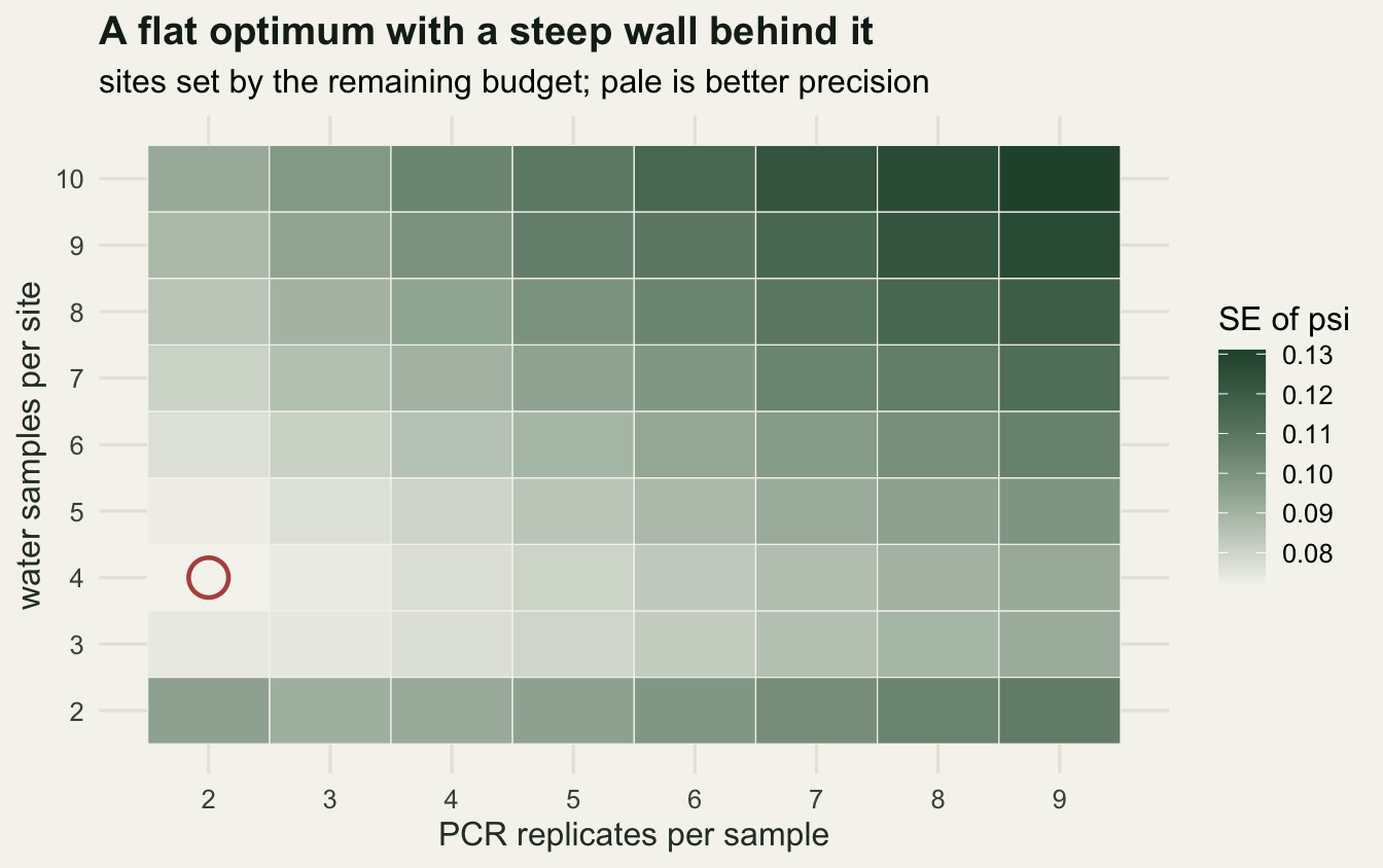

Figure 1: Asymptotic standard error of occupancy over the grid of samples per site and replicates per sample, at a budget of 2000 with the number of sites set by what is left. The best design is ringed.

The tile plot shows why the folklore survives. There is a broad pale plateau and then a steep climb once replicates or samples eat the money that sites needed.

Replicates saturate

The saturation is arithmetic, not statistical. A replicate can only raise the chance of catching a sample that already holds DNA, and that chance is one minus the failure probability raised to the number of replicates, so it approaches its ceiling geometrically. Once it is close, extra wells buy almost nothing while still costing money that could have been a site.

best_at_k <- function(psi, theta, p, budget, n_rep, samp_max = 12) {
  vals <- sapply(2:samp_max, function(j) {
    n_sites <- floor(budget / design_cost(1, j, n_rep))
    if (n_sites < 2) return(NA_real_)
    se_psi(psi, theta, p, n_sites, j, n_rep)
  })
  j_best <- (2:samp_max)[which.min(vals)]
  data.frame(replicates = n_rep, samples = j_best,
             sites = floor(budget / design_cost(1, j_best, n_rep)),
             se = min(vals, na.rm = TRUE))
}

sat <- NULL
for (th in c(0.2, 0.8)) {
  for (pp in c(0.4, 0.7)) {
    rows <- do.call(rbind, lapply(2:9, function(k)
      best_at_k(psi_true, th, pp, budget, k)))
    rows$theta <- th
    rows$p <- pp
    sat <- rbind(sat, rows)
  }
}

for (th in c(0.2, 0.8)) {
  for (pp in c(0.4, 0.7)) {
    sub_rows <- sat[abs(sat$theta - th) < 1e-9 & abs(sat$p - pp) < 1e-9, ]
    k_best <- sub_rows$replicates[which.min(sub_rows$se)]
    cat("theta", th, " p", pp, " SE at two to nine replicates:",
        round(sub_rows$se, 5), "\n   best at", k_best,
        "replicates; nine replicates cost an extra",
        round(100 * (sub_rows$se[sub_rows$replicates == 9] /
                       min(sub_rows$se) - 1), 1), "percent\n")
  }
}

theta 0.2  p 0.4  SE at two to nine replicates: 0.13004 0.1251 0.12599 0.12855 0.13254 0.13836 0.14444 0.14911 
   best at 3 replicates; nine replicates cost an extra 19.2 percent
theta 0.2  p 0.7  SE at two to nine replicates: 0.10913 0.11236 0.11842 0.12438 0.12951 0.13648 0.14349 0.14852 
   best at 2 replicates; nine replicates cost an extra 36.1 percent
theta 0.8  p 0.4  SE at two to nine replicates: 0.06815 0.06497 0.06449 0.06397 0.06499 0.06632 0.06816 0.06975 
   best at 5 replicates; nine replicates cost an extra 9 percent
theta 0.8  p 0.7  SE at two to nine replicates: 0.05733 0.05729 0.05928 0.06116 0.06339 0.06538 0.0676 0.06941 
   best at 3 replicates; nine replicates cost an extra 21.2 percent

With a weak assay (p = 0.4) the curve has a real minimum: three replicates at low sample positivity, five at high positivity. With a good assay (p = 0.7) the minimum has moved down to two or three replicates and the curve climbs from there. Running nine replicates instead of the best number costs from 9 to 36.1 percent of precision depending on the row, all of it spent on wells that were nearly certain to agree with each other.

sat$theta_label <- factor(ifelse(sat$theta < 0.5,
                                 "low sample positivity (theta = 0.2)",
                                 "high sample positivity (theta = 0.8)"),
                          levels = c("low sample positivity (theta = 0.2)",
                                     "high sample positivity (theta = 0.8)"))
sat$p_label <- ifelse(sat$p < 0.55, "weak assay (p = 0.4)",
                      "good assay (p = 0.7)")
minima <- do.call(rbind, lapply(split(sat, list(sat$theta, sat$p)),
                                function(z) z[which.min(z$se), ]))

ggplot(sat, aes(replicates, se, colour = p_label)) +
  geom_line(linewidth = 0.9) +
  geom_point(data = minima, size = 3) +
  facet_wrap(~theta_label, scales = "free_y") +
  scale_colour_manual(values = c(`weak assay (p = 0.4)` = te_pal$clay,
                                 `good assay (p = 0.7)` = te_pal$forest),
                      name = NULL) +
  scale_x_continuous(breaks = 2:9) +
  labs(title = "Past a handful of replicates the money is wasted",
       subtitle = "points mark the best number of replicates in each series",
       x = "PCR replicates per sample", y = "SE of psi") +
  theme_te() +
  theme(legend.position = "top")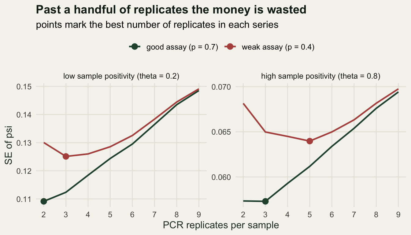

Figure 2: Best achievable standard error of occupancy at each number of PCR replicates, with samples per site and number of sites chosen freely under the same budget of 2000.

What moves the optimum

Two of the three parameters move the answer, and they move it in different directions.

move_tab <- NULL
for (th in c(0.2, 0.8)) {
  top <- design_grid(psi_true, th, p_true, budget)[1, ]
  move_tab <- rbind(move_tab, data.frame(varied = "theta", value = th,
                                         samples = top$samples,
                                         replicates = top$replicates,
                                         sites = top$sites,
                                         se = round(top$se, 4)))
}
for (ps in c(0.1, 0.8)) {
  top <- design_grid(ps, theta_true, p_true, budget)[1, ]
  move_tab <- rbind(move_tab, data.frame(varied = "psi", value = ps,
                                         samples = top$samples,
                                         replicates = top$replicates,
                                         sites = top$sites,
                                         se = round(top$se, 4)))
}
move_tab$site_detection <- round(
  1 - (1 - ifelse(move_tab$varied == "theta", move_tab$value, theta_true) *
         (1 - (1 - p_true)^move_tab$replicates))^move_tab$samples, 4)
print(move_tab, row.names = FALSE)

 varied value samples replicates sites     se site_detection
  theta   0.2       9          2    31 0.1091         0.8360
  theta   0.8       2          3    83 0.0573         0.9509
    psi   0.1       3          2    71 0.0424         0.8381
    psi   0.8       5          2    50 0.0650         0.9519

Sample positivity dominates. At theta = 0.2 the optimum is 31 sites with nine samples each and two replicates; at theta = 0.8 it is 83 sites with two samples each and three replicates. When most water samples from an occupied site contain nothing, the only way to learn that the site is occupied is to take more bottles, and the plate cannot help: a replicate cannot find DNA that is not in the tube. This is the sharpest practical difference between eDNA design and the two-level visit problem, where there is no such level to be starved.

Occupancy moves the optimum much less, and towards more effort per site as the species gets commoner: three samples and 71 sites at psi = 0.1, five samples and 50 sites at psi = 0.8, with the per-site detection probability rising from 0.8381 to 0.9519. The reason is visible in the two contributions to the variance of psi. One is the binomial spread of a proportion, which shrinks as psi leaves 0.5, and the other is the cost of not knowing whether a site with no positives was empty or merely missed. For a rare species the first term is small and most sites are genuinely empty, so extra sites are the better buy; for a common species almost every all-zero site is a candidate false absence and resolving it is what the money is for. The same logic drives the two-level result in the visits tutorial, which is reassuring, because the two calculations share no code.

Designing at a guessed parameter

The optimum is optimal for the parameters you assumed, and those parameters are what the survey exists to estimate. So the honest question is not what the optimum is but how much a wrong guess costs. Fix the design chosen at psi = 0.4 and theta = 0.5, then evaluate it at other truths and compare with the design that would have been chosen there.

excess_curve <- function(vary, values) {
  do.call(rbind, lapply(values, function(v) {
    ps <- if (vary == "psi") v else psi_true
    th <- if (vary == "theta") v else theta_true
    opt <- design_grid(ps, th, p_true, budget)[1, ]
    fixed <- se_psi(ps, th, p_true, best_row$sites, best_row$samples,
                    best_row$replicates)
    data.frame(vary = vary, value = v, opt_samples = opt$samples,
               opt_replicates = opt$replicates,
               excess_pct = round(100 * (fixed / opt$se - 1), 2))
  }))
}

sens <- rbind(excess_curve("psi", seq(0.05, 0.9, by = 0.05)),
              excess_curve("theta", seq(0.15, 0.95, by = 0.05)))
is_psi <- sens$vary == "psi"
cat("worst extra SE from a wrong occupancy guess:",
    max(sens$excess_pct[is_psi]), "percent; over psi up to 0.6 only",
    max(sens$excess_pct[is_psi & sens$value < 0.61]), "percent\n")

worst extra SE from a wrong occupancy guess: 17.23 percent; over psi up to 0.6 only 0.52 percent

cat("worst extra SE from a wrong positivity guess:",
    max(sens$excess_pct[!is_psi]), "percent\n")

worst extra SE from a wrong positivity guess: 65.25 percent

print(sens[round(sens$value, 2) %in% c(0.05, 0.15, 0.6, 0.9), ],
      row.names = FALSE)

  vary value opt_samples opt_replicates excess_pct
   psi  0.05           3              2       0.52
   psi  0.15           4              2       0.00
   psi  0.60           5              2       0.44
   psi  0.90           7              2      17.23
 theta  0.15          10              2      65.25
 theta  0.60           3              2       2.52
 theta  0.90           2              2      19.90

Guessing occupancy wrong is close to free over the range a survey is usually in. Up to psi = 0.6 the design chosen at psi = 0.4 loses at most 0.52 percent of precision, and its worst case anywhere in 0.05 to 0.9 is 17.23 percent, at the far end where the species occupies nine sites in ten. Guessing sample positivity wrong is expensive: at a true theta of 0.15 the design chosen at 0.5 gives a standard error 65.25 percent larger than the achievable one, because it took four bottles where it needed ten.

That asymmetry is the useful design advice in this post. A pilot study that only pins down rough occupancy has bought little; a pilot that measures how often a bottle from a known-occupied site tests positive has bought most of what the design needs.

sens$panel <- factor(ifelse(sens$vary == "psi",
                            "occupancy psi (design assumed 0.4)",
                            "sample positivity theta (design assumed 0.5)"),
                     levels = c("occupancy psi (design assumed 0.4)",
                                "sample positivity theta (design assumed 0.5)"))

ggplot(sens, aes(value, excess_pct)) +
  geom_hline(yintercept = 0, colour = te_pal$line) +
  geom_line(colour = te_pal$forest, linewidth = 0.9) +
  geom_point(colour = te_pal$forest, size = 1.8) +
  facet_wrap(~panel, scales = "free_x") +
  labs(title = "A wrong positivity guess costs far more than a wrong psi",
       subtitle = "extra SE of psi against the best design available at that truth",
       x = "true value of the parameter",
       y = "extra SE (percent)") +
  theme_te()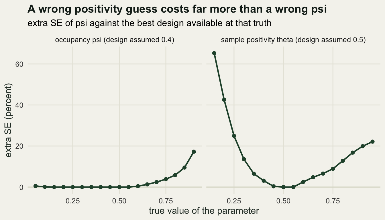

Figure 3: Extra standard error incurred by the design chosen at psi = 0.4 and theta = 0.5 when the true value differs, relative to the best design at each true value.

Scoring the three-replicate rule

Field protocols routinely recommend three PCR replicates per sample, and the tile plot suggests the rule is not bad. Measure it: for each pair of assumed theta and p, compare the best design overall with the best design that is forced to three replicates.

folklore <- NULL
for (th in c(0.2, 0.35, 0.5, 0.8)) {
  for (pp in c(0.4, 0.55, 0.7, 0.9)) {
    gr <- design_grid(psi_true, th, pp, budget)
    forced <- gr[gr$replicates == 3, ][1, ]
    folklore <- rbind(folklore, data.frame(
      theta = th, p = pp, best_replicates = gr$replicates[1],
      best_samples = gr$samples[1], best_se = round(gr$se[1], 4),
      rule_samples = forced$samples, rule_se = round(forced$se, 4),
      loss_pct = forced$excess_pct))
  }
}
print(folklore, row.names = FALSE)

 theta    p best_replicates best_samples best_se rule_samples rule_se loss_pct
  0.20 0.40               3           10  0.1251           10  0.1251     0.00
  0.20 0.55               3           10  0.1157           10  0.1157     0.00
  0.20 0.70               2            9  0.1091           10  0.1124     2.96
  0.20 0.90               2            9  0.1045           10  0.1112     6.41
  0.35 0.40               3            6  0.0962            6  0.0962     0.00
  0.35 0.55               2            7  0.0896            6  0.0896     0.05
  0.35 0.70               2            6  0.0842            5  0.0866     2.90
  0.35 0.90               2            5  0.0805            5  0.0855     6.12
  0.50 0.40               4            4  0.0812            5  0.0814     0.23
  0.50 0.55               3            4  0.0756            4  0.0756     0.00
  0.50 0.70               2            4  0.0716            4  0.0736     2.82
  0.50 0.90               2            4  0.0693            4  0.0729     5.29
  0.80 0.40               5            2  0.0640            3  0.0650     1.57
  0.80 0.55               3            2  0.0598            2  0.0598     0.00
  0.80 0.70               3            2  0.0573            2  0.0573     0.00
  0.80 0.90               2            2  0.0545            2  0.0565     3.68

cat("worst loss from the three-replicate rule:", max(folklore$loss_pct),
    "percent, median loss:", median(folklore$loss_pct), "percent\n")

worst loss from the three-replicate rule: 6.41 percent, median loss: 0.9 percent

cat("cells where the rule is exactly optimal:",
    sum(folklore$loss_pct < 0.005), "of", nrow(folklore), "\n")

cells where the rule is exactly optimal: 6 of 16 

The rule is close to optimal over most of this table. Its worst cell loses 6.41 percent of precision, the median loss is 0.9 percent, and it is exactly optimal in six of the sixteen cells. It fails in one direction only, towards a good assay: at p = 0.9 the third replicate is nearly redundant and the loss runs from 3.68 to 6.41 percent depending on theta. Against the flatness of the optimum and the uncertainty in theta, a fixed rule of three replicates costs less than a bad guess at sample positivity does, which is a fair defence of the folklore.

What the optimum does not know

Three limits, and none of them is small.

The design depends on parameters the survey is meant to estimate. The sensitivity measured above bounds the damage for psi and for theta separately at this cost ratio, but a design optimised at a guess is not a design with a guarantee, and the loss from a wrong theta was large enough to change what a pilot study should measure.

The cost model is a caricature. Travel is not linear in the number of sites: a route that visits 58 sites is cheaper per site than one that visits five, and a remote site can cost more than a whole plate. Replicates come in steps because a plate has a fixed number of wells, so the grid above has affordable designs on it that no lab would run. Substituting realistic costs is easy; the point is that the answer is a function of them, and reporting an optimum without the cost ratios is not reproducible.

Minimising the standard error of psi is a choice, not the only objective. A survey that only needs to know whether a species is present anywhere in a catchment should maximise the probability of at least one detection, which pushes towards fewer sites sampled harder, and a survey comparing two areas needs the standard error of a difference instead. Each objective has its own optimum on the same grid, which is cheap to re-score once the information matrix is in hand.

Where to go next

The next tutorial in this cluster turns the machinery on a finished analysis rather than a planned one: what to check before believing a three-level eDNA occupancy fit, how to tell a boundary estimate from a real one, and which of the diagnostics from the single-season occupancy world still apply when the detection process has two nested layers.

References

Guillera-Arroita G, Lahoz-Monfort JJ 2012 Methods in Ecology and Evolution 3(5):860-869 (10.1111/j.2041-210X.2012.00225.x)

MacKenzie DI, Royle JA 2005 Journal of Applied Ecology 42(6):1105-1114 (10.1111/j.1365-2664.2005.01098.x)

Bailey LL, Hines JE, Nichols JD, MacKenzie DI 2007 Ecological Applications 17(1):281-290 (10.1890/1051-0761(2007)017[0281:SDTIOS]2.0.CO;2)

Dorazio RM, Erickson RA 2018 Molecular Ecology Resources 18(2):368-380 (10.1111/1755-0998.12735)

Related tutorials

• Three-level occupancy models for eDNA
• False positives in eDNA surveys
• How many visits? Occupancy survey design
• Checking an eDNA occupancy analysis