Three-level occupancy models for eDNA

An eDNA survey can miss a species at three levels. Fit site occupancy, sample availability and PCR detection by hand in R, and see what pooling them costs.

An eDNA survey has three chances to miss a species that is there. The site can be occupied and the water sample can still carry no target DNA, because the animal was elsewhere in the pond that morning or the DNA had already degraded. The sample can carry DNA and a PCR replicate can still fail to amplify it. Only the last of these is what a standard occupancy model calls detection, and the middle one has nowhere to go in a two-level likelihood.

This tutorial simulates the full hierarchy with known parameters, writes the three-level likelihood out by hand, and measures what ignoring the middle level does to the estimates. The quantity a survey protocol is actually chosen on comes out at the end: the probability of detecting the species at an occupied site, given a number of water samples and a number of PCR replicates per sample.

Three chances to miss

Three parameters, one per level. Site occupancy psi is the probability that a site holds the species. Availability theta is the probability that a water sample from an occupied site contains detectable target DNA. Detection p is the probability that one PCR replicate from a DNA-bearing sample amplifies. The data are counts of positive replicates per sample, not per site.

library(ggplot2)

te_pal <- list(forest = "#275139", green = "#2f8f63", sage = "#93a87f",
               clay = "#b5534e", gold = "#cda23f", line = "#dad9ca",
               ink = "#16241d", paper = "#f5f4ee")

theme_te <- function() {
  theme_minimal(base_size = 12) +
    theme(panel.grid.minor = element_blank(),
          panel.grid.major = element_line(colour = "#e7e6dc"),
          plot.background = element_rect(fill = "#f5f4ee", colour = NA),
          panel.background = element_rect(fill = "#f5f4ee", colour = NA),
          plot.title = element_text(face = "bold", colour = te_pal$ink),
          axis.title = element_text(colour = "#2c3a31"))
}

n_sites <- 120
n_samp <- 5
n_rep <- 8
psi_true <- 0.6
theta_true <- 0.5
p_true <- 0.7

cat("truth: psi", psi_true, " theta", theta_true, " p", p_true, "\n")

truth: psi 0.6  theta 0.5  p 0.7 

cat("design:", n_sites, "sites,", n_samp, "water samples per site,", n_rep,
    "PCR replicates per sample\n")

design: 120 sites, 5 water samples per site, 8 PCR replicates per sample

set.seed(501)
occ_true <- rbinom(n_sites, 1, psi_true)
avail <- matrix(rbinom(n_sites * n_samp, 1, theta_true), n_sites, n_samp) *
  occ_true
y_obs <- matrix(rbinom(n_sites * n_samp, n_rep, p_true), n_sites, n_samp) * avail
site_tot <- rowSums(y_obs)
occ_rows <- occ_true == 1

cat("occupied sites in the truth:", sum(occ_true),
    " realised fraction:", round(mean(occ_true), 4),
    " sites with at least one positive replicate:", sum(site_tot > 0), "\n")

occupied sites in the truth: 64  realised fraction: 0.5333  sites with at least one positive replicate: 60 

cat("share of samples from occupied sites with no positive replicate:",
    round(mean(y_obs[occ_rows, ] == 0), 4),
    " occupied sites missed entirely:", sum(occ_rows & site_tot == 0), "\n")

share of samples from occupied sites with no positive replicate: 0.475  occupied sites missed entirely: 4 

cat("mean positive replicates out of", n_rep, "among samples that amplified:",
    round(mean(y_obs[y_obs > 0]), 4), "\n")

mean positive replicates out of 8 among samples that amplified: 5.5417 

Almost half the samples taken at occupied sites, 0.475 of them, produced nothing at all, while the samples that did amplify averaged 5.5417 positives out of 8. That gap is the signature of the middle level. Failure is not spread thinly across replicates; it arrives in whole samples, and within a sample that worked the replicates mostly agree.

Four of the 64 occupied sites produced no positive replicate anywhere, so the naive count already misses some. The more interesting damage is not the missed sites.

show_n <- 24
struct_df <- data.frame(
  site = rep(seq_len(show_n), times = n_samp),
  water_sample = rep(seq_len(n_samp), each = show_n),
  positives = as.vector(y_obs[seq_len(show_n), ]),
  state = ifelse(rep(occ_true[seq_len(show_n)], times = n_samp) == 1,
                 "site occupied", "site empty"))

ggplot(struct_df, aes(factor(water_sample), factor(site), fill = positives)) +
  geom_tile(colour = "#f5f4ee", linewidth = 0.6, width = 1, height = 1) +
  geom_text(aes(label = positives, colour = positives > 4), size = 2.9) +
  facet_grid(state ~ ., scales = "free_y", space = "free_y") +
  scale_fill_gradient(low = "#e2e0cf", high = te_pal$forest,
                      name = "positive replicates") +
  scale_colour_manual(values = c(`FALSE` = te_pal$ink, `TRUE` = te_pal$paper),
                      guide = "none") +
  labs(title = "Whole samples fail, not single replicates",
       subtitle = "positive PCR replicates out of eight, first 24 sites",
       x = "water sample", y = "site") +
  theme_te() +
  theme(panel.grid = element_blank(), axis.text.y = element_text(size = 8),
        legend.position = "bottom")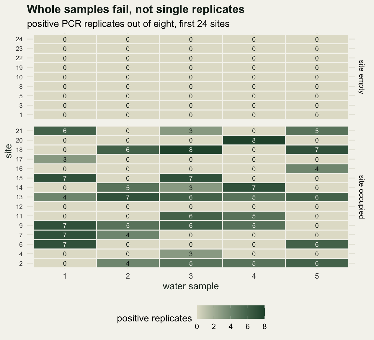

Figure 1: Positive PCR replicates out of eight in each water sample, for the first twenty-four simulated sites, split by the true occupancy state. Empty sites are all zero by construction because this simulation has no contamination.

The likelihood, one site at a time

Two sets of latent variables have to go: the occupancy state of each site and the availability state of each sample. There are 2^(J + 1) combinations of them per site, which sounds expensive, but the samples are conditionally independent given occupancy, so the sum collapses into a product of two-term sums.

For an occupied site, a sample with y positives out of K replicates contributes theta * dbinom(y, K, p) + (1 - theta) * (y == 0): either the sample held DNA and the replicates behaved binomially, or it did not and the only possible observation is a row of zeros. An unoccupied site contributes 1 if every count is zero and 0 otherwise. The site likelihood is psi times the product over samples, plus 1 - psi times the indicator that the whole site was negative.

site_loglik <- function(psi, theta, prob, ymat, k_rep) {
  samp_term <- theta * dbinom(ymat, k_rep, prob) + (1 - theta) * (ymat == 0)
  occ_part <- exp(rowSums(log(samp_term)))
  log(psi * occ_part + (1 - psi) * (rowSums(ymat) == 0))
}

nll_three <- function(par, ymat, k_rep) {
  pr <- plogis(par)
  val <- -sum(site_loglik(pr[1], pr[2], pr[3], ymat, k_rep))
  if (is.finite(val)) val else 1e10
}

nll_two <- function(par, tot, n_visit) {
  pr <- plogis(par)
  val <- -sum(log(pr[1] * dbinom(tot, n_visit, pr[2]) +
                    (1 - pr[1]) * (tot == 0)))
  if (is.finite(val)) val else 1e10
}

det_site <- function(theta, prob, j_samp, k_rep) {
  1 - (1 - theta * (1 - (1 - prob)^k_rep))^j_samp
}

fit_probs <- function(fn, start, ...) {
  fit <- optim(start, fn, ..., method = "BFGS", hessian = TRUE,
               control = list(maxit = 500))
  est <- plogis(fit$par)
  se_logit <- sqrt(diag(solve(fit$hessian)))
  data.frame(estimate = est, se = est * (1 - est) * se_logit)
}

All three parameters are fitted on the logit scale so that optim runs unconstrained, and the standard errors come from the numerically differentiated Hessian that optim returns, pushed back to the probability scale by the delta method: the derivative of the inverse logit is est * (1 - est). Using dbinom adds a binomial coefficient that does not depend on any parameter, so it shifts the log-likelihood by a constant and changes nothing about the estimates.

three <- fit_probs(nll_three, c(0, 0, 0), ymat = y_obs, k_rep = n_rep)
three_tab <- data.frame(parameter = c("psi", "theta", "p"),
                        truth = c(psi_true, theta_true, p_true),
                        estimate = round(three$estimate, 4),
                        se = round(three$se, 4))
print(three_tab, row.names = FALSE)

 parameter truth estimate     se
       psi   0.6   0.5094 0.0466
     theta   0.5   0.5497 0.0303
         p   0.7   0.6927 0.0126

Availability comes back at 0.5497 against a true 0.5, and replicate detection at 0.6927 against 0.7. Occupancy comes back at 0.5094 with a standard error of 0.0466, which looks low against 0.6 until you notice that only 64 of the 120 sites were actually occupied in this draw, a realised fraction of 0.5333. A single data set of this size cannot resolve a bias of a percentage point or two, which is why the comparison below is repeated.

Three estimators, one data set

The naive estimator calls a site occupied if any replicate anywhere came back positive. The two-level model does what most published analyses do with this kind of data: it treats the 40 PCR replicates from a site as 40 independent visits and fits the standard occupancy likelihood to their total. The three-level model keeps the sample level.

naive_psi <- mean(site_tot > 0)
naive_se <- sqrt(naive_psi * (1 - naive_psi) / n_sites)
pooled <- fit_probs(nll_two, c(0, 0), tot = site_tot, n_visit = n_samp * n_rep)

comp <- data.frame(
  estimator = c("naive", "two-level pooled", "two-level pooled",
                "three-level", "three-level", "three-level"),
  parameter = c("psi", "psi", "p", "psi", "theta", "p"),
  truth = c(psi_true, psi_true, p_true, psi_true, theta_true, p_true),
  estimate = round(c(naive_psi, pooled$estimate, three$estimate), 4),
  se = round(c(naive_se, pooled$se, three$se), 4))
print(comp, row.names = FALSE)

        estimator parameter truth estimate     se
            naive       psi   0.6   0.5000 0.0456
 two-level pooled       psi   0.6   0.5000 0.0456
 two-level pooled         p   0.7   0.3879 0.0099
      three-level       psi   0.6   0.5094 0.0466
      three-level     theta   0.5   0.5497 0.0303
      three-level         p   0.7   0.6927 0.0126

nll_corner <- function(par, ymat, k_rep) {
  pr <- plogis(par)
  -sum(site_loglik(pr[1], 1, pr[2], ymat, k_rep))
}
corner <- optim(c(0, 0), nll_corner, ymat = y_obs, k_rep = n_rep,
                method = "BFGS")
cat("forcing theta to 1 gives psi and p:", round(plogis(corner$par), 4), "\n")

forcing theta to 1 gives psi and p: 0.5 0.3879 

cat("log-likelihood at the three-level maximum:",
    round(-nll_three(qlogis(three$estimate), y_obs, n_rep), 2),
    " with theta forced to 1:", round(-corner$value, 2),
    " difference:", round(-nll_three(qlogis(three$estimate), y_obs, n_rep) +
                            corner$value, 2), "\n")

log-likelihood at the three-level maximum: -590.36  with theta forced to 1: -1159.26  difference: 568.89 

cat("probability of detecting the species at an occupied site under the truth:",
    round(det_site(theta_true, p_true, n_samp, n_rep), 4),
    " limit of the naive estimator:",
    round(psi_true * det_site(theta_true, p_true, n_samp, n_rep), 4), "\n")

probability of detecting the species at an occupied site under the truth: 0.9687  limit of the naive estimator: 0.5812 

Occupancy survives the pooling almost intact here, 0.5 against 0.5094, and the reason is in the last line: with five samples of eight replicates the probability of detecting the species at an occupied site is 0.9687, so the naive estimator converges to 0.5812 rather than 0.6 and there is very little for a model to recover. Detection does not survive. Pooled per-replicate detection comes out at 0.3879 against a true 0.7, barely half.

The mechanism is a misallocation of the zeros. A pooled model has one way to explain a zero, a replicate that failed, so the 0.475 of samples that came back empty, nearly all of them because they never contained DNA, are counted as long runs of failed replicates and detection is dragged down to match. The link is exact rather than approximate: forcing theta to 1 in the three-level likelihood, which is precisely the assumption that every sample from an occupied site contains DNA, returns psi 0.5 and p 0.3879, the pooled estimates to four decimals. That corner of the parameter space sits 568.89 log-likelihood units below the interior maximum, so the data reject it about as clearly as data can reject anything.

one_run <- function() {
  z <- rbinom(n_sites, 1, psi_true)
  av <- matrix(rbinom(n_sites * n_samp, 1, theta_true), n_sites, n_samp) * z
  yy <- matrix(rbinom(n_sites * n_samp, n_rep, p_true), n_sites, n_samp) * av
  tt <- rowSums(yy)
  f2 <- optim(c(0, 0), nll_two, tot = tt, n_visit = n_samp * n_rep,
              method = "BFGS")
  f3 <- optim(c(0, 0, 0), nll_three, ymat = yy, k_rep = n_rep, method = "BFGS")
  c(mean(tt > 0), plogis(f2$par[1]), plogis(f2$par[2]),
    plogis(f3$par[1]), plogis(f3$par[2]), plogis(f3$par[3]))
}

set.seed(502)
sims <- t(sapply(seq_len(200), function(i) one_run()))
cat("simulated data sets:", nrow(sims), "\n")

simulated data sets: 200 

rep_tab <- data.frame(
  quantity = c("naive psi", "pooled psi", "pooled p", "three-level psi",
               "three-level theta", "three-level p"),
  truth = c(psi_true, psi_true, p_true, psi_true, theta_true, p_true),
  mean_estimate = round(colMeans(sims), 4),
  sd_estimate = round(apply(sims, 2, sd), 4))
print(rep_tab, row.names = FALSE)

          quantity truth mean_estimate sd_estimate
         naive psi   0.6        0.5858      0.0469
        pooled psi   0.6        0.5858      0.0469
          pooled p   0.7        0.3613      0.0188
   three-level psi   0.6        0.6057      0.0485
 three-level theta   0.5        0.4986      0.0294
     three-level p   0.7        0.7013      0.0124

Two hundred data sets from the same truth separate luck from bias. Naive and pooled occupancy both average 0.5858, close to the 0.5812 that the algebra predicts for the naive estimator, while the three-level estimator averages 0.6057 around a truth of 0.6. Pooled detection averages 0.3613, and the three-level estimates of availability and detection average 0.4986 and 0.7013.

lab_par <- c(psi = "site occupancy psi", p = "per-replicate detection p")
keep <- comp$parameter %in% c("psi", "p")
est_df <- rbind(
  data.frame(estimator = comp$estimator[keep], parameter = comp$parameter[keep],
             estimate = comp$estimate[keep],
             lower = comp$estimate[keep] - comp$se[keep],
             upper = comp$estimate[keep] + comp$se[keep],
             source = "one data set, model standard error"),
  data.frame(estimator = c("naive", "two-level pooled", "two-level pooled",
                           "three-level", "three-level"),
             parameter = c("psi", "psi", "p", "psi", "p"),
             estimate = rep_tab$mean_estimate[c(1, 2, 3, 4, 6)],
             lower = rep_tab$mean_estimate[c(1, 2, 3, 4, 6)] -
               rep_tab$sd_estimate[c(1, 2, 3, 4, 6)],
             upper = rep_tab$mean_estimate[c(1, 2, 3, 4, 6)] +
               rep_tab$sd_estimate[c(1, 2, 3, 4, 6)],
             source = "200 simulations, standard deviation"))
est_df$panel <- factor(lab_par[est_df$parameter],
                       levels = as.character(lab_par))
est_df$estimator <- factor(est_df$estimator,
                           levels = c("naive", "two-level pooled",
                                      "three-level"))
truth_df <- data.frame(panel = factor(as.character(lab_par),
                                      levels = as.character(lab_par)),
                       truth = c(psi_true, p_true))

ggplot(est_df, aes(estimator, estimate, colour = source)) +
  geom_hline(data = truth_df, aes(yintercept = truth),
             linetype = "dashed", colour = "grey40") +
  geom_errorbar(aes(ymin = lower, ymax = upper), width = 0.14, linewidth = 0.7,
                position = position_dodge(width = 0.5)) +
  geom_point(size = 2.6, position = position_dodge(width = 0.5)) +
  facet_wrap(~panel, scales = "free_y") +
  scale_colour_manual(values = c(te_pal$clay, te_pal$forest), name = NULL) +
  labs(title = "Pooling the sample level halves detection",
       subtitle = "dashed: the values that generated the data",
       x = NULL, y = "estimate") +
  theme_te() +
  theme(legend.position = "bottom",
        axis.text.x = element_text(angle = 12, hjust = 1))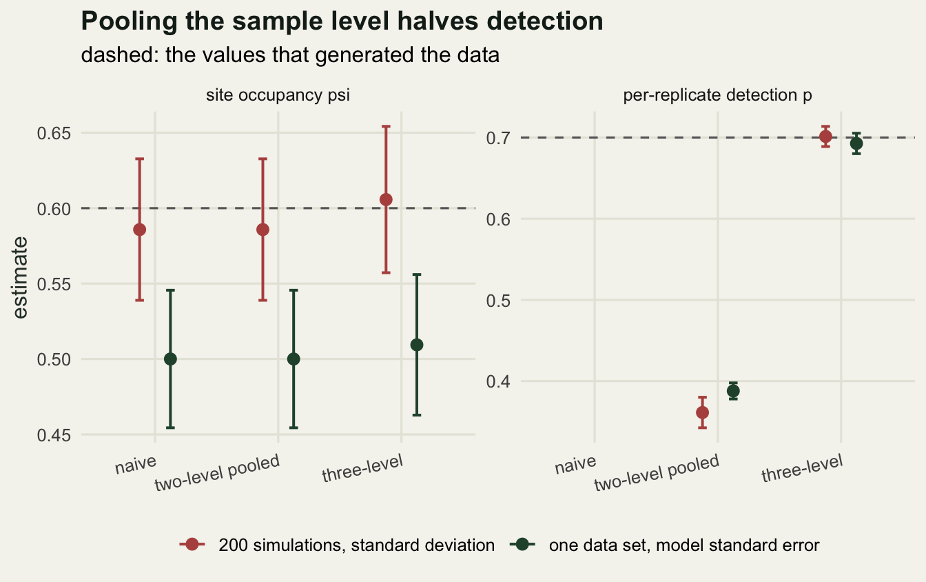

Figure 2: Site occupancy and per-replicate detection from three estimators, shown for the single data set with its model standard error and as the mean over 200 simulated data sets with its standard deviation. Dashed lines are the true 0.6 and 0.7.

What the protocol implies

None of this matters much for a map of occupancy, which is why pooled analyses get away with it. It matters for design, because the number a protocol is chosen on is the probability of detecting the species at an occupied site, and that number is built from all three levels: 1 - (1 - theta * (1 - (1 - p)^K))^J for J samples of K replicates.

est_theta <- three$estimate[2]
est_p <- three$estimate[3]
cat("fitted detection at an occupied site, five samples of eight replicates:",
    round(det_site(est_theta, est_p, n_samp, n_rep), 4), "\n")

fitted detection at an occupied site, five samples of eight replicates: 0.9815 

grid_small <- outer(c(1, 2, 3, 5, 8), c(1, 2, 3, 5, 8),
                    function(j, k) round(det_site(est_theta, est_p, j, k), 3))
dimnames(grid_small) <- list(samples = c(1, 2, 3, 5, 8),
                             replicates = c(1, 2, 3, 5, 8))
print(grid_small)

       replicates
samples     1     2     3     5     8
      1 0.381 0.498 0.534 0.548 0.550
      2 0.617 0.748 0.783 0.796 0.797
      3 0.763 0.873 0.899 0.908 0.909
      5 0.909 0.968 0.978 0.981 0.981
      8 0.978 0.996 0.998 0.998 0.998

cat("one water sample with eight replicates: three-level model",
    round(det_site(est_theta, est_p, 1, n_rep), 4),
    " pooled two-level model", round(1 - (1 - pooled$estimate[2])^n_rep, 4),
    "\n")

one water sample with eight replicates: three-level model 0.5496  pooled two-level model 0.9803 

prot_df <- expand.grid(replicates = 1:10, samples = 1:6)
prot_df$detection <- det_site(est_theta, est_p, prot_df$samples,
                              prot_df$replicates)
reach <- prot_df[prot_df$detection >= 0.95, ]
reach$reactions <- reach$samples * reach$replicates
reach <- reach[order(reach$reactions), ]
reach$detection <- round(reach$detection, 4)
cat("cheapest designs reaching 0.95 detection at an occupied site:\n")

cheapest designs reaching 0.95 detection at an occupied site:

print(head(reach, 3), row.names = FALSE)

 replicates samples detection reactions
          2       5    0.9680        10
          3       4    0.9527        12
          2       6    0.9839        12

Read the grid down a column rather than along a row. Adding replicates to one water sample buys almost nothing past the third: one sample rises from 0.381 to 0.534 and then stalls at 0.550, because no number of PCR replicates can find DNA that the bottle never contained. Adding samples works, and the trade is worth pricing: five samples of two replicates reach 0.968 for 10 reactions in total, the cheapest design in the grid that clears 0.95. Four samples of three replicates get there as well, for 12.

This is where the pooled model does real harm. Asked what one water sample with eight replicates achieves, it answers 0.9803, because it thinks every replicate is an independent look at the site. The three-level model answers 0.5496. A protocol designed on the first number samples one bottle per pond and misses half the occupied ponds.

ggplot(prot_df, aes(replicates, samples)) +
  geom_tile(aes(fill = detection), colour = "#f5f4ee", linewidth = 0.5) +
  geom_text(aes(label = sprintf("%.2f", detection),
                colour = detection > 0.85), size = 2.7) +
  geom_contour(aes(z = detection), breaks = 0.95, colour = te_pal$clay,
               linewidth = 0.9) +
  scale_fill_gradient(low = "#e2e0cf", high = te_pal$forest,
                      name = "detection") +
  scale_colour_manual(values = c(`FALSE` = te_pal$ink, `TRUE` = te_pal$paper),
                      guide = "none") +
  scale_x_continuous(breaks = 1:10) +
  scale_y_continuous(breaks = 1:6) +
  labs(title = "Samples buy detection, replicates do not",
       subtitle = "probability of detecting the species at an occupied site",
       x = "PCR replicates per sample", y = "water samples per site") +
  theme_te() +
  theme(panel.grid = element_blank())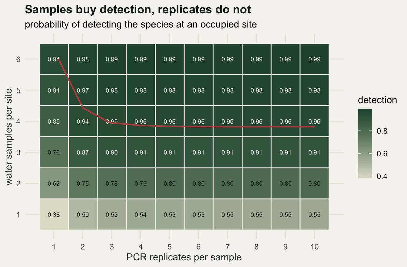

Figure 3: Probability of detecting the species at an occupied site, at the fitted availability and detection, over a grid of water samples and PCR replicates. The line marks 0.95.

Where availability and detection stop being separable

The three-level model needs the replicates to disagree with each other sometimes. With a single PCR replicate per sample, a sample is positive with probability theta * p and negative with probability 1 - theta * p, and nothing in the data can say which of the two factors is small. Simulate that design and profile the likelihood to see it.

set.seed(503)
occ_k1 <- rbinom(n_sites, 1, psi_true)
avail_k1 <- matrix(rbinom(n_sites * n_samp, 1, theta_true), n_sites, n_samp) *
  occ_k1
y_k1 <- matrix(rbinom(n_sites * n_samp, 1, p_true), n_sites, n_samp) * avail_k1
cat("single-replicate design: sites with at least one positive sample:",
    sum(rowSums(y_k1) > 0), " the product theta times p in the truth:",
    round(theta_true * p_true, 4), "\n")

single-replicate design: sites with at least one positive sample: 66  the product theta times p in the truth: 0.35 

prof_split <- function(theta_val, q_val, ymat, k_rep) {
  obj <- function(psi) -sum(site_loglik(psi, theta_val, q_val / theta_val,
                                        ymat, k_rep))
  -optimize(obj, c(0.02, 0.999))$objective
}
prof_product <- function(q_val, ymat, k_rep) {
  obj <- function(par) {
    th <- q_val + (1 - q_val) * plogis(par[2])
    -sum(site_loglik(plogis(par[1]), th, q_val / th, ymat, k_rep))
  }
  -optim(c(0, 0), obj, method = "Nelder-Mead")$value
}

fit_k1 <- optim(c(0, 0, 0), nll_three, ymat = y_k1, k_rep = 1, method = "BFGS")
q_k1 <- prod(plogis(fit_k1$par[2:3]))
q_k8 <- est_theta * est_p
cat("product at the maximum: one replicate", round(q_k1, 4),
    " eight replicates", round(q_k8, 4), "\n")

product at the maximum: one replicate 0.3637  eight replicates 0.3807 

prof_line <- function(ymat, k_rep, q_val) {
  th <- seq(q_val + 0.02, 0.99, length.out = 41)
  data.frame(theta = th,
             loglik = sapply(th, function(x) prof_split(x, q_val, ymat, k_rep)))
}
pl1 <- prof_line(y_k1, 1, q_k1)
pl8 <- prof_line(y_obs, n_rep, q_k8)
cat("one replicate, profile log-likelihood at theta", round(pl1$theta[1], 2),
    "and", round(pl1$theta[41], 2), ":", round(pl1$loglik[1], 2), "and",
    round(pl1$loglik[41], 2), "\n")

one replicate, profile log-likelihood at theta 0.38 and 0.99 : -299.45 and -299.45 

cat("eight replicates, the same two ends:", round(pl8$loglik[1], 2), "and",
    round(pl8$loglik[41], 2), " maximum at theta",
    round(pl8$theta[which.max(pl8$loglik)], 4), "\n")

eight replicates, the same two ends: -1058.57 and -1109.61  maximum at theta 0.548 

flat_width <- function(pl) {
  ok <- pl$loglik >= max(pl$loglik) - 1.92
  diff(range(pl$theta[ok]))
}
cat("width in theta of the region within 1.92 log-likelihood units:",
    " one replicate", round(flat_width(pl1), 4),
    " eight replicates", round(flat_width(pl8), 4), "\n")

width in theta of the region within 1.92 log-likelihood units:  one replicate 0.6063  eight replicates 0.0295 

q_grid <- seq(0.15, 0.6, by = 0.01)
pq1 <- sapply(q_grid, function(q) prof_product(q, y_k1, 1))
in_ci <- q_grid[pq1 >= max(pq1) - 1.92]
cat("one replicate, profile interval for the product:", round(min(in_ci), 4),
    "to", round(max(in_ci), 4), "\n")

one replicate, profile interval for the product: 0.31 to 0.42 

Fix the product at its maximum and walk along it, trading availability against detection. With one replicate per sample the profile log-likelihood is -299.45 at both ends of the walk, at availability 0.38 and at 0.99: identical to two decimals, and flat across the whole range the product allows, a width of 0.6063. With eight replicates the same walk drops from -1058.57 to -1109.61 and the region within 1.92 log-likelihood units of the maximum is 0.0295 wide, twenty times narrower.

What the single-replicate design does estimate is the product. Its profile interval runs from 0.31 to 0.42, comfortably around the true 0.35, and its maximum sits at 0.3637. The information is there; it just cannot be split.

set.seed(504)
starts <- matrix(rnorm(3 * 40, 0, 1.5), 40, 3)
ridge <- function(ymat, k_rep, label) {
  out <- t(apply(starts, 1, function(s) {
    fit <- optim(s, nll_three, ymat = ymat, k_rep = k_rep, method = "BFGS")
    c(plogis(fit$par), fit$value)
  }))
  colnames(out) <- c("psi", "theta", "p", "nll")
  ok <- out[, 4] <= min(out[, 4]) + 0.01
  cat(label, "fits reaching the maximum:", sum(ok), "of", nrow(out),
      " theta from", round(min(out[ok, 2]), 4), "to",
      round(max(out[ok, 2]), 4), " p from", round(min(out[ok, 3]), 4), "to",
      round(max(out[ok, 3]), 4), "\n")
  cat(label, "product from", round(min(out[ok, 2] * out[ok, 3]), 4), "to",
      round(max(out[ok, 2] * out[ok, 3]), 4), " correlation of theta and p:",
      round(cor(out[ok, 2], out[ok, 3]), 4), "\n")
  if (any(!ok)) {
    cat(label, "fits stuck short of the maximum:\n")
    print(round(out[!ok, 1:3, drop = FALSE], 4))
  }
}
ridge(y_k1, 1, "one replicate:")

one replicate: fits reaching the maximum: 40 of 40  theta from 0.3656 to 0.9733  p from 0.3737 to 0.9949 
one replicate: product from 0.3636 to 0.3638  correlation of theta and p: -0.965 

ridge(y_obs, n_rep, "eight replicates:")

eight replicates: fits reaching the maximum: 38 of 40  theta from 0.5496 to 0.5498  p from 0.6926 to 0.6927 
eight replicates: product from 0.3807 to 0.3808  correlation of theta and p: -0.1968 
eight replicates: fits stuck short of the maximum:
     psi theta      p
[1,] 1.0  0.28 0.6927
[2,] 0.5  1.00 0.3879

The same thing from the optimiser’s side. Start the single-replicate fit from 40 random points and all 40 reach the same maximised log-likelihood, with availability anywhere from 0.3656 to 0.9733 and detection from 0.3737 to 0.9949, correlated at -0.965, while the product stays between 0.3636 and 0.3638. The data cannot choose among those fits; only the starting point can. With eight replicates, 38 of the 40 starts reach the maximum and they agree on availability from 0.5496 to 0.5498. The two stuck fits are printed above and both sit in a corner: one at availability 1, which is the pooled model, the other at occupancy 1 with availability 0.28, which explains the sites with no positives as sampling failure instead of absence. Corners are where the gradient vanishes, so a fit that reports a probability of exactly 1 should be restarted rather than believed.

What the model does not tell you

The estimates above are about DNA. A site here is occupied if its water carries target sequence, and the model has no way to ask whether the animal is present, was present last month, or is upstream of the sampling point. Every ecological reading of psi inherits that gap, and calling it site occupancy does not close it.

Constant availability and constant detection are the other real restriction. Inhibition varies between samples, the volume filtered varies, distance from the source varies, and any of those breaks the assumption that all samples from a site share one theta and all replicates share one p. The consequence is not a small loss of efficiency; heterogeneity in availability behaves like a further mixture, and fitting a single theta to a mixture of good and bad samples biases the design calculation in the direction that flatters the protocol.

False positives are assumed away here. The simulation gives an unoccupied site zero chance of a positive replicate, which is exactly what a contaminated bench does not do, and a single false positive in the wrong place can move an occupancy estimate more than all the detection modelling above.

Where to go next

The next tutorial in this cluster puts contamination into the same likelihood and measures what a small per-replicate false positive rate does to psi. It assumes this post, and both assume the two tutorials that build the machinery: the single-season occupancy likelihood and the general nested multi-scale model, which is the same structure in a non-molecular setting.

References

Schmidt BR, Kery M, Ursenbacher S, Hyman OJ, Collins JP 2013 Methods in Ecology and Evolution 4(7):646-653 (10.1111/2041-210X.12052)

Dorazio RM, Erickson RA 2018 Molecular Ecology Resources 18(2):368-380 (10.1111/1755-0998.12735)

Nichols JD et al 2008 Journal of Applied Ecology 45(5):1321-1329 (10.1111/j.1365-2664.2008.01509.x)

Mordecai RS, Mattsson BJ, Tzilkowski CJ, Cooper RJ 2011 Journal of Applied Ecology 48(1):56-66 (10.1111/j.1365-2664.2010.01921.x)

Related tutorials

• Multi-scale occupancy models in R
• Fitting single-season occupancy models in R
• False positives in eDNA surveys
• Checking an eDNA occupancy analysis