---
title: "Multi-scale occupancy models in R"
description: "A nested occupancy model separates site use, local availability and detection. Skip the middle scale and a single-scale fit quietly underestimates occupancy."
date: "2026-05-23 13:00"
categories: [occupancy, detection, hierarchical models, monitoring, ecology tutorial]
image: thumbnail.png
image-alt: "Dot and whisker chart in one panel with four labelled categories on an estimate axis with ticks from 0.4 to 0.7: three dark green points with vertical error bars, and a fourth amber point at the right for the naive estimate, also with error bars, sitting near 0.37. A short red horizontal dash marks the target of each estimate, and the fourth dash is drawn at psi times theta, about 0.39, so the amber point sits just below it and its interval covers it."
---
Many surveys are nested. A landscape is split into sites, each site holds several stations or subunits, and each subunit is visited a few times. A species can be present in the site as a whole yet use only some of the subunits, and even where it is present it is not always detected. That gives three probabilities stacked on top of one another: site occupancy, local use given occupancy, and per-visit detection. A single-scale occupancy model has room for only two of them, so it folds the first two together and reports something that is neither.
This post fits the nested model in base R, shows what the naive single-scale fit actually estimates, and confirms it with a small simulation study.
## The nested process
Let psi be the probability a site is occupied, theta the probability a subunit is used given the site is occupied, and p the per-visit detection probability. A subunit yields detections only when its site is occupied, the subunit is used, and the species is seen.
```{r setup}
#| code-fold: true
#| code-summary: "Setup: packages, colours and plot theme"
#| results: hide
#| message: false
#| warning: false
knitr::opts_chunk$set(echo = TRUE, message = FALSE, warning = FALSE,
                      fig.width = 7.5, fig.height = 4.6, dpi = 150, dev = "png")
library(ggplot2)
te <- list(ink="#16241d", body="#2c3a31", forest="#275139", label="#46604a",
           sage="#93a87f", paper="#f5f4ee", line="#dad9ca", card="#ffffff",
           faint="#5d6b61", grazed="#cda23f", mown="#2f8f63", abandoned="#b5534e",
           grad_low="#c9b458", grad_high="#1d5b4e")
theme_te <- function(base_size = 12) {
  theme_minimal(base_size = base_size) +
    theme(text=element_text(colour=te$body),
          plot.title=element_text(colour=te$ink, face="bold", size=base_size+1),
          plot.subtitle=element_text(colour=te$faint, size=base_size-1),
          axis.title=element_text(colour=te$label),
          axis.text=element_text(colour=te$faint, size=base_size-2),
          panel.grid.major=element_line(colour=te$line, linewidth=0.3),
          panel.grid.minor=element_blank(),
          panel.background=element_rect(fill=te$paper, colour=NA),
          plot.background=element_rect(fill=te$paper, colour=NA),
          legend.title=element_text(colour=te$label, size=base_size-2),
          legend.text=element_text(colour=te$faint, size=base_size-2),
          strip.text=element_text(colour=te$ink, face="bold", size=base_size-1),
          strip.background=element_rect(fill=te$paper, colour=NA),
          plot.margin=margin(10,12,10,10))
}
```
```{r simulate}
set.seed(1)
R <- 150      # sites
J <- 4        # subunits per site
K <- 3        # visits per subunit
psi_true <- 0.70; theta_true <- 0.55; p_true <- 0.45

z <- rbinom(R, 1, psi_true)                       # site occupied
a <- matrix(rbinom(R * J, 1, theta_true), R, J)   # subunit used given site
a <- a * z                                        # use requires occupancy
D <- matrix(0L, R, J)                             # detections out of K per subunit
for (i in 1:R) for (j in 1:J) D[i, j] <- rbinom(1, K, a[i, j] * p_true)
c(sites_occupied = sum(z), subunits_detected = sum(D > 0), n_subunits = R * J)
```
## The marginal likelihood
We cannot observe the latent states, so we sum them out. For one subunit the probability of its detection count given that it is used is a binomial term; given that it is not used the count must be zero. A site's contribution multiplies the subunit terms, weighted by whether the site is occupied at all.
```{r fit-multiscale}
nll_ms <- function(par) {
  psi <- plogis(par[1]); theta <- plogis(par[2]); p <- plogis(par[3])
  pu   <- p^D * (1 - p)^(K - D)          # subunit history given used
  zero <- (D == 0)                        # subunit history if not used
  inner <- theta * pu + (1 - theta) * zero
  prod_inner <- apply(inner, 1, prod)     # site occupied
  all_zero   <- apply(zero,  1, prod)     # site empty implies all subunits silent
  ll <- log(psi * prod_inner + (1 - psi) * all_zero)
  -sum(ll)
}
fit_ms <- optim(c(0, 0, 0), nll_ms, method = "BFGS", hessian = TRUE)
stopifnot(fit_ms$convergence == 0)   # check before inverting the Hessian
est_ms <- plogis(fit_ms$par)
V  <- solve(fit_ms$hessian)                # covariance on the logit scale
lo <- plogis(fit_ms$par - 1.96 * sqrt(diag(V)))
hi <- plogis(fit_ms$par + 1.96 * sqrt(diag(V)))
names(est_ms) <- c("psi", "theta", "p")
round(rbind(estimate = est_ms, lower = lo, upper = hi), 3)
```
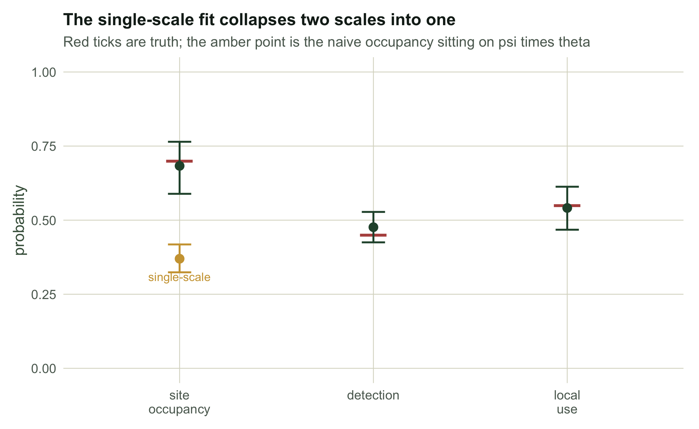
The nested fit recovers all three probabilities: site occupancy is `r round(est_ms[1], 3)` (truth `r psi_true`), local use is `r round(est_ms[2], 3)` (truth `r theta_true`), and detection is `r round(est_ms[3], 3)` (truth `r p_true`). Each confidence interval covers its true value.
## What the single-scale fit estimates
Now drop the middle scale. Treat every subunit as an independent site with one occupancy probability q and the same detection p. This is the ordinary two-level occupancy model most people reach for first.
```{r fit-naive}
nll_naive <- function(par) {
  q <- plogis(par[1]); p <- plogis(par[2])
  pu   <- p^D * (1 - p)^(K - D)
  zero <- (D == 0)
  ll <- log(q * pu + (1 - q) * zero)     # every subunit treated independently
  -sum(ll)
}
fit_naive <- optim(c(0, 0), nll_naive, method = "BFGS", hessian = TRUE)
q_naive <- plogis(fit_naive$par[1]); p_naive <- plogis(fit_naive$par[2])
c(q_naive = round(q_naive, 3), product_psi_theta = round(psi_true * theta_true, 3),
  p_naive = round(p_naive, 3))
```
The single-scale occupancy comes out at `r round(q_naive, 3)`, which sits right on the product psi times theta, `r round(psi_true * theta_true, 3)`. That is exactly what it targets: the marginal probability that any one subunit is used. Read as site occupancy it understates the truth by about `r round(100 * (1 - q_naive / psi_true))` per cent. Detection is still fine, because the naive model gets the visit-level part right; it is only the occupancy number that is quietly the wrong quantity.
```{r}
#| label: fig-estimates
#| fig-cap: "Nested estimates against their truths, with the single-scale occupancy for comparison. The naive value lands on the product of site occupancy and local use."
#| fig-alt: "Points with error bars for site occupancy, local use and detection near their true tick marks, and a separate naive occupancy point sitting on the product of the first two."
tk <- data.frame(par = c("site\noccupancy", "local\nuse", "detection"),
                 truth = c(psi_true, theta_true, p_true))
dm <- data.frame(par = factor(tk$par, levels = tk$par),
                 est = est_ms, lo = lo, hi = hi)
dn <- data.frame(par = factor("site\noccupancy", levels = tk$par),
                 est = q_naive,
                 lo = plogis(fit_naive$par[1] - 1.96 * sqrt(solve(fit_naive$hessian)[1, 1])),
                 hi = plogis(fit_naive$par[1] + 1.96 * sqrt(solve(fit_naive$hessian)[1, 1])))
ggplot(dm, aes(par, est)) +
  geom_point(data = tk, aes(par, truth), shape = 95, size = 12, colour = te$abandoned) +
  geom_errorbar(aes(ymin = lo, ymax = hi), width = 0.12, colour = te$forest, linewidth = 0.7) +
  geom_point(size = 2.8, colour = te$forest) +
  geom_errorbar(data = dn, aes(ymin = lo, ymax = hi), width = 0.12, colour = te$grazed, linewidth = 0.7) +
  geom_point(data = dn, size = 2.8, colour = te$grazed) +
  annotate("text", x = 1, y = q_naive - 0.06, label = "single-scale", colour = te$grazed, size = 3.2) +
  scale_y_continuous(limits = c(0, 1)) +
  labs(x = NULL, y = "probability",
       title = "The single-scale fit collapses two scales into one",
       subtitle = "Red ticks are truth; the amber point is the naive occupancy sitting on psi times theta") +
  theme_te()
```
## A check across data sets
To be sure the pattern is not a fluke of one simulation, we regenerate the data many times and store the four estimates each time.
```{r mc}
sim_fit <- function(seed) {
  set.seed(seed)
  zz <- rbinom(R, 1, psi_true)
  aa <- matrix(rbinom(R * J, 1, theta_true), R, J) * zz
  DD <- matrix(rbinom(R * J, K, as.numeric(aa) * p_true), R, J)
  nms <- function(par) { ps<-plogis(par[1]);th<-plogis(par[2]);p<-plogis(par[3])
    pu<-p^DD*(1-p)^(K-DD); ze<-(DD==0); inr<-th*pu+(1-th)*ze
    -sum(log(ps*apply(inr,1,prod)+(1-ps)*apply(ze,1,prod))) }
  nnv <- function(par) { q<-plogis(par[1]);p<-plogis(par[2])
    pu<-p^DD*(1-p)^(K-DD); ze<-(DD==0); -sum(log(q*pu+(1-q)*ze)) }
  fm <- tryCatch(optim(c(0,0,0), nms, method="BFGS"), error=function(e) NULL)
  fn <- tryCatch(optim(c(0,0),   nnv, method="BFGS"), error=function(e) NULL)
  if (is.null(fm) || is.null(fn)) return(rep(NA, 4))
  c(plogis(fm$par), plogis(fn$par[1]))
}
M  <- 200
mc <- t(sapply(1:M, function(m) sim_fit(2000 + m)))
mc <- mc[stats::complete.cases(mc), ]
colnames(mc) <- c("psi", "theta", "p", "naive_q")
round(rbind(mean = colMeans(mc), sd = apply(mc, 2, sd)), 3)
```
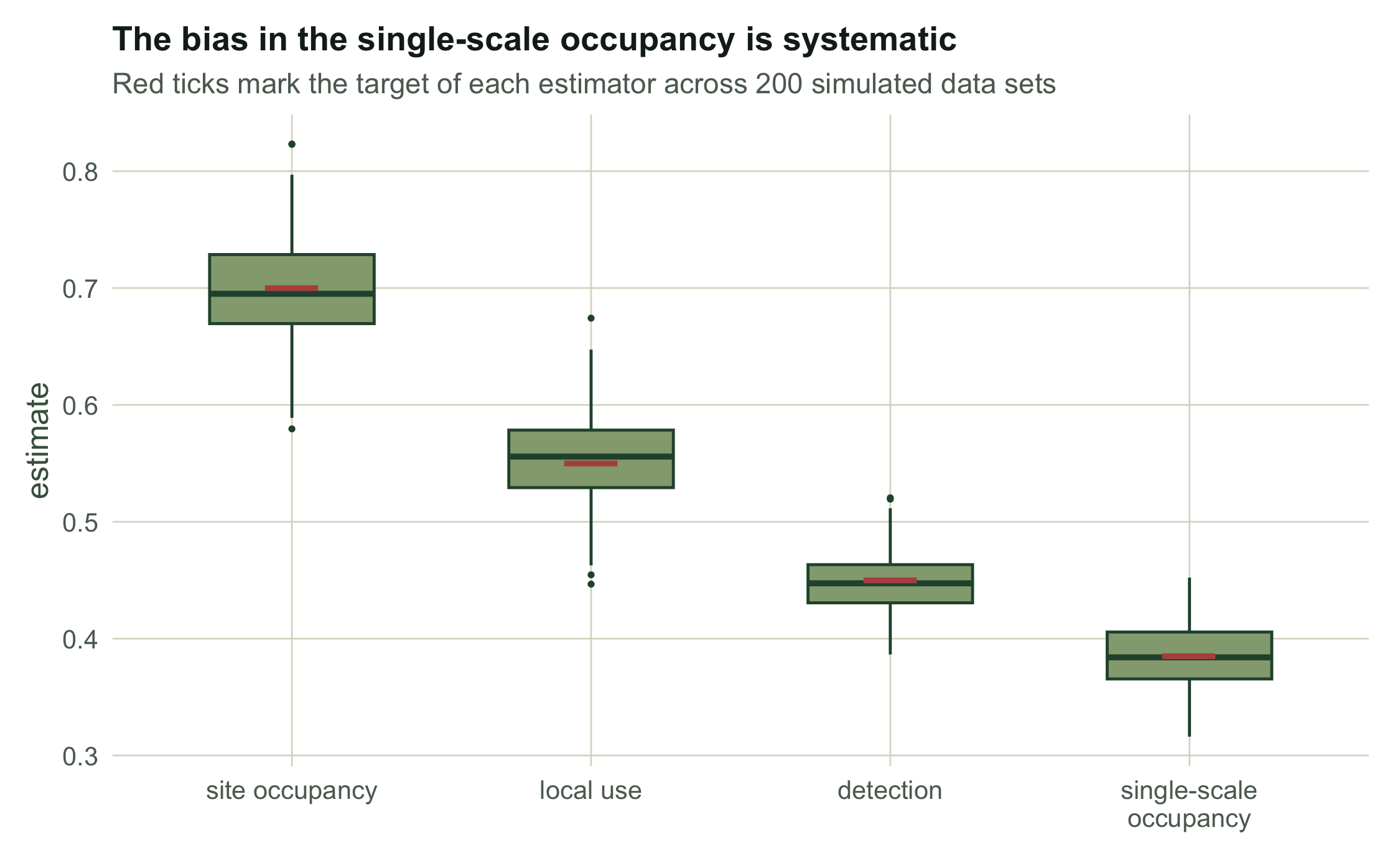
Over `r nrow(mc)` data sets the nested estimates are unbiased, centred on `r round(mean(mc[,"psi"]), 2)`, `r round(mean(mc[,"theta"]), 2)` and `r round(mean(mc[,"p"]), 2)`. The single-scale occupancy averages `r round(mean(mc[,"naive_q"]), 3)`, again the product of the two upper probabilities rather than site occupancy itself. The bias is systematic, not random: more visits or more sites will not remove it, because the estimator is answering a different question.
```{r}
#| label: fig-boxplots
#| fig-cap: "Sampling distributions across simulations. The nested estimates straddle their truths; the single-scale occupancy is centred on the product."
#| fig-alt: "Boxplots for the three nested estimates near their true lines and the naive occupancy centred well below the true site occupancy line."
long <- data.frame(
  value = c(mc[,"psi"], mc[,"theta"], mc[,"p"], mc[,"naive_q"]),
  which = rep(c("site occupancy", "local use", "detection", "single-scale\noccupancy"), each = nrow(mc)))
long$which <- factor(long$which, levels = c("site occupancy", "local use", "detection", "single-scale\noccupancy"))
tru <- data.frame(which = levels(long$which),
                  t = c(psi_true, theta_true, p_true, psi_true * theta_true))
tru$which <- factor(tru$which, levels = levels(long$which))
ggplot(long, aes(which, value)) +
  geom_boxplot(fill = te$sage, colour = te$forest, outlier.size = 0.6, width = 0.55) +
  geom_point(data = tru, aes(which, t), shape = 95, size = 12, colour = te$abandoned) +
  labs(x = NULL, y = "estimate",
       title = "The bias in the single-scale occupancy is systematic",
       subtitle = "Red ticks mark the target of each estimator across 200 simulated data sets") +
  theme_te()
```
## The takeaway
If your design has a level of spatial structure between the site and the visit, that level belongs in the model. The nested model needs no more data than you already collected; it just reads it correctly, returning site occupancy and local use as separate numbers. Without a middle level the two subunit-scale states are not separable, and the reported occupancy is the product of the two, which will always look lower than the truth.
## References
MacKenzie DI, Nichols JD, Lachman GB, Droege S, Royle JA, Langtimm CA 2002 Ecology 83:2248-2255 (10.1890/0012-9658(2002)083[2248:ESORWD]2.0.CO;2)
Nichols JD, Bailey LL, O'Connell AF, Talancy NW, Campbell Grant EH, Gilbert AT, Annand EM, Husband TP, Hines JE 2008 Journal of Applied Ecology 45:1321-1329 (10.1111/j.1365-2664.2008.01509.x)
Mordecai RS, Mattsson BJ, Tzilkowski CJ, Cooper RJ 2011 Journal of Applied Ecology 48:56-66 (10.1111/j.1365-2664.2010.01921.x)
Pavlacky DC, Blakesley JA, White GC, Hanni DJ, Lukacs PM 2012 Journal of Wildlife Management 76:154-162 (10.1002/jwmg.245)
## Related tutorials
- [Logistic regression for presence-absence](../logistic-regression-presence-absence/)
- [Spatial autocorrelation in occupancy](../spatial-autocorrelation-in-occupancy/)
- [Checking an integrated SDM](../checking-an-integrated-sdm/)
- [Three-level occupancy models for eDNA](../edna-occupancy-three-levels/)