Spatial autocorrelation in occupancy models

A latent spatial gradient in occupancy inflates false positives for any structured covariate. Moran eigenvector filtering restores honest standard errors.

Occupancy models assume that, once the covariates are in the model, the sites are conditionally independent. Real landscapes rarely oblige. Nearby sites share unmeasured drivers such as soil, drainage or history, so occupancy is spatially smooth in ways no covariate captures. That leftover structure does not just sit quietly in the residuals: if any predictor is itself spatially patterned, the model can mistake the shared smoothness for a real effect, and it does so with badly overconfident standard errors.

This post shows the problem with a covariate that has no true effect, then fixes it with restricted spatial regression using Moran eigenvectors, all in base R.

A lattice with a hidden gradient

We work on a square lattice. Occupancy is driven by a smooth latent field that we never give the model. A second covariate is also spatially smooth but has no effect on occupancy at all. It is a pure null: any slope the model assigns to it is a false positive.

# a smooth field on a g x g grid, standardised
smooth_field <- function(g, l, seed) {
  set.seed(seed)
  u <- (seq_len(g) - 0.5) / g
  D <- outer(u, u, function(a, b) exp(-(a - b)^2 / (2 * l^2)))
  Sm <- D / rowSums(D)
  as.numeric(scale(as.numeric(Sm %*% matrix(rnorm(g * g), g, g) %*% t(Sm))))
}

g <- 16; R <- g * g; K <- 4; p_true <- 0.5
cx <- rep((seq_len(g) - 0.5) / g, times = g)
cy <- rep((seq_len(g) - 0.5) / g, each = g)

# rook adjacency: neighbours share an edge
idx <- matrix(1:R, g, g); W <- matrix(0, R, R)
for (r in 1:g) for (c in 1:g) {
  h <- idx[r, c]
  if (r > 1) W[h, idx[r - 1, c]] <- 1; if (r < g) W[h, idx[r + 1, c]] <- 1
  if (c > 1) W[h, idx[r, c - 1]] <- 1; if (c < g) W[h, idx[r, c + 1]] <- 1
}

# Moran's I for a vector on this lattice
moran <- function(z, W) {
  z <- z - mean(z)
  (length(z) / sum(W)) * sum(W * outer(z, z)) / sum(z^2)
}

The spatial filter comes from the eigenvectors of the doubly centred adjacency matrix. These eigenvectors are orthogonal spatial patterns ordered from broad trends to fine checkerboards; adding a handful of the broad ones to the model gives it a flexible spatial term without any covariance parameters to estimate.

q <- 30                                   # number of spatial eigenvectors to offer
one <- rep(1, R)
Cmat <- diag(R) - outer(one, one) / R     # double-centring operator
ev <- eigen(Cmat %*% W %*% Cmat, symmetric = TRUE)
Esel <- ev$vectors[, 1:q, drop = FALSE]   # the broadest spatial patterns

sig_s <- 1.6; sf_len <- 0.20; x0_len <- 0.08
field <- sig_s * smooth_field(g, sf_len, 101)   # latent driver of occupancy (hidden)
x0    <- smooth_field(g, x0_len, 101 + 5000)     # spatially patterned null covariate
set.seed(101)
z <- rbinom(R, 1, plogis(field))                 # true occupancy from the field alone
y <- rbinom(R, K, z * p_true)                    # detections over K visits
c(true_occupancy = round(mean(plogis(field)), 3), ever_detected = sum(y > 0), sites = R)

true_occupancy  ever_detected          sites 
         0.487        119.000        256.000 

Fitting with and without a spatial term

The occupancy likelihood marginalises the latent presence state. We fit it twice: once with just the null covariate, and once with the null covariate plus the spatial eigenvectors.

nll <- function(par, Xd, y, K) {
  np <- ncol(Xd); psi <- plogis(Xd %*% par[1:np]); p <- plogis(par[np + 1])
  -sum(log(psi * dbinom(y, K, p) + (1 - psi) * (y == 0)))
}
fit <- function(Xd, y, K) {
  np <- ncol(Xd)
  f <- optim(c(rep(0, np), 0), nll, Xd = Xd, y = y, K = K, method = "BFGS", hessian = TRUE)
  se <- tryCatch(sqrt(diag(solve(f$hessian))), error = function(e) rep(NA, np + 1))
  list(f = f, se = se, np = np)
}
Xn <- cbind(1, x0);        mn <- fit(Xn, y, K)          # naive
Xr <- cbind(1, x0, Esel);  mr <- fit(Xr, y, K)          # RSR filtered
bN <- mn$f$par[2]; sN <- mn$se[2]
bR <- mr$f$par[2]; sR <- mr$se[2]

# Pearson residuals on the detection scale and their Moran's I
resid_p <- function(m, Xd) {
  np <- m$np; psi <- plogis(Xd %*% m$f$par[1:np]); p <- plogis(m$f$par[np + 1])
  pi <- psi * (1 - (1 - p)^K); o <- as.numeric(y > 0); (o - pi) / sqrt(pi * (1 - pi))
}
rN <- as.numeric(resid_p(mn, Xn)); rR <- as.numeric(resid_p(mr, Xr))
miN <- moran(rN, W); miR <- moran(rR, W)
round(c(b_naive = bN, se_naive = sN, moran_naive = miN,
        b_rsr = bR, se_rsr = sR, moran_rsr = miR), 3)

    b_naive    se_naive moran_naive       b_rsr      se_rsr   moran_rsr 
      0.087       0.134       0.214      -0.566       0.465      -0.078 

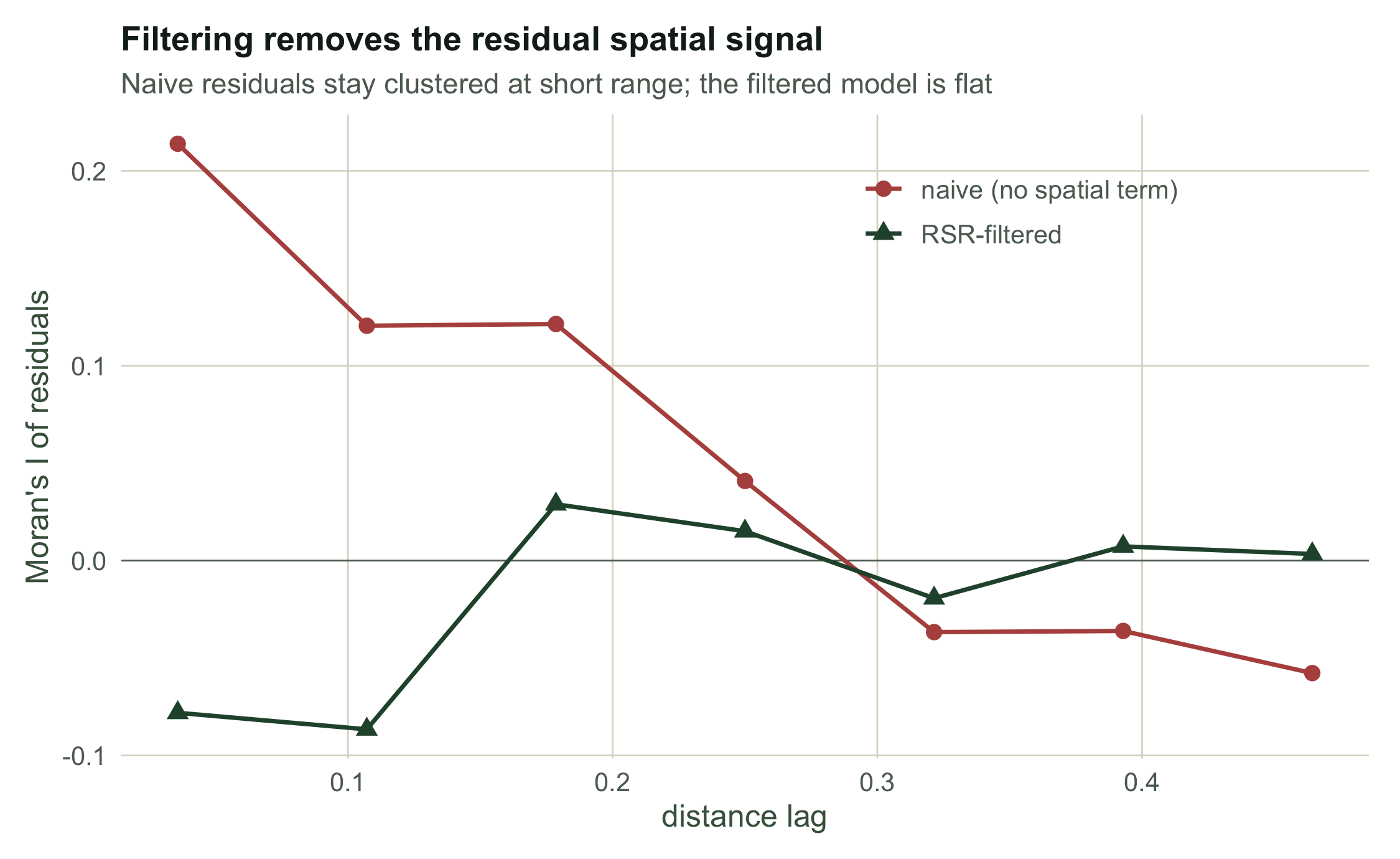
On this one data set neither model happens to call the null covariate significant. The tell is elsewhere. The naive residuals are still spatially clustered, with a Moran’s I of 0.214, because the model has nothing to absorb the hidden gradient. After filtering, residual autocorrelation drops to -0.078, essentially zero. The price is honesty about uncertainty: the standard error on the null slope widens from 0.134 to 0.465, a factor of about 3.47. The naive model was that overconfident.

dxy <- as.matrix(dist(cbind(cx, cy))); brks <- seq(0, 0.5, length.out = 8)
corl <- function(rv) sapply(1:(length(brks) - 1), function(b) {
  Wb <- (dxy > brks[b] & dxy <= brks[b + 1]) * 1
  if (sum(Wb) == 0) return(NA); moran(rv, Wb)
})
lag <- (brks[-1] + brks[-length(brks)]) / 2
cg <- data.frame(lag = rep(lag, 2), I = c(corl(rN), corl(rR)),
                 model = rep(c("naive (no spatial term)", "RSR-filtered"), each = length(lag)))
ggplot(cg, aes(lag, I, colour = model, shape = model)) +
  geom_hline(yintercept = 0, colour = te$faint, linewidth = 0.3) +
  geom_line(linewidth = 0.8) + geom_point(size = 2.6) +
  scale_colour_manual(values = c("naive (no spatial term)" = te$abandoned, "RSR-filtered" = te$forest)) +
  scale_shape_manual(values = c("naive (no spatial term)" = 16, "RSR-filtered" = 17)) +
  labs(x = "distance lag", y = "Moran's I of residuals",
       title = "Filtering removes the residual spatial signal",
       subtitle = "Naive residuals stay clustered at short range; the filtered model is flat",
       colour = NULL, shape = NULL) +
  theme_te() + theme(legend.position = c(0.72, 0.85))

Figure 1: Residual Moran’s I by distance lag. The naive model leaves autocorrelation at short distances; the filtered model is flat near zero.

The false-positive rate

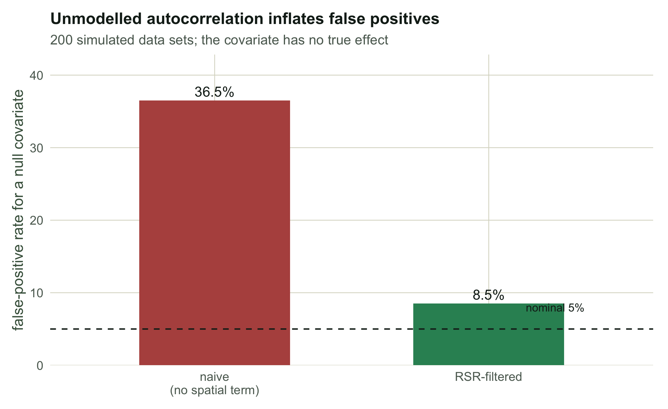
A single data set cannot show a rate. We simulate many, each with a fresh latent field and a fresh null covariate, and count how often each model calls the null slope significant at the five per cent level.

fit_b <- function(Xd, y, K) {
  np <- ncol(Xd)
  f <- optim(c(rep(0, np), 0), nll, Xd = Xd, y = y, K = K, method = "BFGS", hessian = TRUE)
  se <- tryCatch(sqrt(diag(solve(f$hessian)))[2], error = function(e) NA)
  c(f$par[2], se)
}
M <- 200; out <- matrix(NA, M, 2)
for (m in 1:M) {
  s  <- sig_s * smooth_field(g, sf_len, 7000 + m)
  x0m <- smooth_field(g, x0_len, 13000 + m)
  zz <- rbinom(R, 1, plogis(s)); yy <- rbinom(R, K, zz * p_true)
  a <- fit_b(cbind(1, x0m), yy, K)
  b <- fit_b(cbind(1, x0m, Esel), yy, K)
  out[m, ] <- c(a[1] / a[2], b[1] / b[2])
}
tiN <- 100 * mean(abs(out[, 1]) > 1.96, na.rm = TRUE)
tiR <- 100 * mean(abs(out[, 2]) > 1.96, na.rm = TRUE)
c(naive_type_I = round(tiN, 1), rsr_type_I = round(tiR, 1), nominal = 5)

naive_type_I   rsr_type_I      nominal 
        36.5          8.5          5.0 

The naive occupancy model rejects the true null about 36 per cent of the time, seven times the nominal five. The filter cuts that to roughly 8 per cent. The improvement is large, and it comes purely from letting the model account for spatial structure rather than pretending it away.

d2 <- data.frame(model = factor(c("naive\n(no spatial term)", "RSR-filtered"),
                                levels = c("naive\n(no spatial term)", "RSR-filtered")),
                 rate = c(tiN, tiR))
ggplot(d2, aes(model, rate, fill = model)) +
  geom_col(width = 0.55) +
  geom_hline(yintercept = 5, colour = te$ink, linetype = "dashed") +
  annotate("text", x = 2.35, y = 8, label = "nominal 5%", hjust = 1, size = 3.2, colour = te$ink) +
  geom_text(aes(label = sprintf("%.1f%%", rate)), vjust = -0.4, size = 4, colour = te$ink) +
  scale_fill_manual(values = c("naive\n(no spatial term)" = te$abandoned, "RSR-filtered" = te$mown), guide = "none") +
  scale_y_continuous(limits = c(0, 42), expand = expansion(mult = c(0, 0.02))) +
  labs(x = NULL, y = "false-positive rate for a null covariate",
       title = "Unmodelled autocorrelation inflates false positives",
       subtitle = "200 simulated data sets; the covariate has no true effect") +
  theme_te()

Figure 2: False-positive rate for a null covariate across 200 simulations. The naive model rejects far too often; filtering brings it close to nominal.

An honest caveat

The filter is not a cure-all. It brings the false-positive rate down to about 8 per cent, better than 36 but still above five. When a covariate and the latent field vary on similar broad scales, the spatial term and the covariate compete for the same signal, and some inflation survives. This is spatial confounding: separating a broad covariate effect from a broad spatial trend is genuinely hard, and no filter can fully manufacture information the data do not contain. Treat the eigenvector approach as a strong correction, report the widened standard errors it gives, and stay cautious about covariates whose pattern mirrors the landscape.

Related tutorials

• Spatial autocorrelation and Moran’s I
• GLS for spatially correlated data
• Multi-scale occupancy models
• Logistic regression for presence-absence

References

Moran PAP (1950) Biometrika 37: 17-23.

Dray S, Legendre P, Peres-Neto PR (2006) Ecological Modelling 196: 483-493.

Griffith DA, Peres-Neto PR (2006) Ecology 87: 2603-2613. doi:10.1890/0012-9658(2006)87[2603:SMIETF]2.0.CO;2

Dormann CF, McPherson JM, Araujo MB, et al. (2007) Ecography 30: 609-628. doi:10.1111/j.2007.0906-7590.05171.x

Hodges JS, Reich BJ (2010) The American Statistician 64: 325-334. doi:10.1198/tast.2010.10052

## References

Moran PAP 1950 Biometrika 37(1-2):17-23 (10.1093/biomet/37.1-2.17)