---
title: "Model-based unconstrained ordination"
description: "An NMDS axis can track sampling intensity rather than ecology when the mean-variance link is strong. A model-based ordination on residuals recovers it."
date: "2026-06-04 09:00"
categories: [R, community ecology, multivariate, ordination, ecology tutorial]
image: thumbnail.png
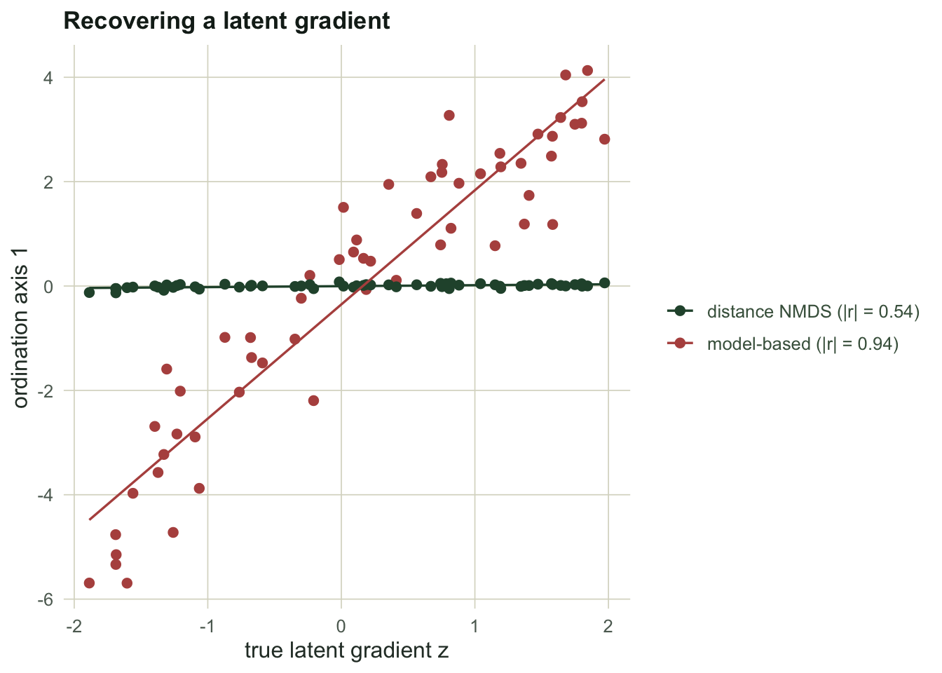
image-alt: "A single scatter plot of standardised ordination axis 1 against the true latent gradient z, with two overlaid point clouds and a fitted line for each. The red cloud rises steeply from about minus 2 to plus 1.5 and stays close to its fitted line, while the green cloud scatters widely about a shallower line, so the red series tracks the gradient far more tightly."
date-modified: "2026-10-14"
---
*Corrected 14 October 2026: the closing paragraph credited the common residual scale alone with bringing the gradient onto the first axis; it now credits the site term that absorbs total abundance together with that scale.*
*Corrected 1 October 2026: the closing paragraph said that putting species on a common residual scale pulls the real gradient back into view; it now says that the first NMDS axis tracked total abundance while the gradient sat on a diagonal of the NMDS plane, and that the residual scale brought it onto the first axis. The stress paragraph no longer says the NMDS faithfully preserved the dissimilarity ranks, only their broad rank order.*
*Corrected 27 September 2026: the gradient-recovery figure drew both ordination axes on one raw scale, so the NMDS axis looked flat on zero and its alt text said it did not track the gradient; both axes are now standardised, and the NMDS points follow the gradient loosely (|r| = 0.54), as the correlation table says.*
Non-metric multidimensional scaling is how most community ecologists look at their data: turn the site-by-species table into Bray-Curtis dissimilarities, squeeze them into two dimensions, and read the picture. It is an algorithm for preserving the rank order of dissimilarities, and it works hard at that. What it does not do is account for the statistical properties of counts, and that omission has a cost. Because Bray-Curtis is dominated by the most abundant species, and because abundance and variance travel together, the first axis often ends up tracking how many individuals were caught rather than which species were there.
A model-based ordination starts from the other end. Fit a generalised linear model to the table, with a site effect that absorbs total abundance and a species effect that absorbs how common each species is, then ordinate what is left over: the Dunn-Smyth residuals. Those residuals live on a common scale for every species, so a rare informative species counts as much as a common uninformative one. This post recovers a known gradient with both methods and shows the difference.
```{r setup}
#| message: false
#| warning: false
#| code-fold: true
#| code-summary: "Setup: packages, colours and plot theme"
library(MASS)
library(ggplot2)

te_ink   <- "#16241d"; te_body <- "#2c3a31"; te_green <- "#275139"
te_label <- "#46604a"; te_sage <- "#93a87f"; te_paper <- "#f5f4ee"
te_line  <- "#dad9ca"; te_faint <- "#5d6b61"; te_warm <- "#b5534e"; te_gold <- "#c9b458"
theme_te <- function() {
  theme_minimal(base_size = 12) +
    theme(panel.grid.minor = element_blank(),
          panel.grid.major = element_line(colour = "#dad9ca", linewidth = 0.3),
          axis.title = element_text(colour = "#2c3a31"),
          axis.text  = element_text(colour = "#5d6b61"),
          plot.title = element_text(colour = "#16241d", face = "bold", size = 13),
          plot.subtitle = element_text(colour = "#46604a", size = 10),
          strip.text = element_text(colour = "#275139", face = "bold"),
          legend.title = element_text(colour = "#2c3a31"),
          legend.text  = element_text(colour = "#46604a"),
          plot.background  = element_rect(fill = "#f5f4ee", colour = NA),
          panel.background = element_rect(fill = "#f5f4ee", colour = NA))
}
```
## A gradient hidden behind sampling intensity
We simulate 60 sites and 25 species. A single latent gradient `z` drives composition, but the species that respond most strongly to it are the rarer ones; the abundant species that dominate a dissimilarity barely track it. On top of that, sites differ in sampling intensity, a multiplier on every species that has nothing to do with ecology. This is the situation where the two approaches part company.
```{r data}
set.seed(4223)
n <- 60; S <- 25
z <- runif(n, -2, 2)                          # true latent gradient (unknown to the methods)
b0     <- sort(rnorm(S, mean = log(c(rep(16,6), rep(5,7), rep(1.6,7), rep(0.7,5))), sd = 0.2),
               decreasing = TRUE)
lambda <- c(rnorm(6, 0, 0.05), rnorm(7, 0, 0.5), rnorm(7, 0, 1.1), rnorm(5, 0, 1.3))
theta_true <- 1.5
samp <- rnorm(n, 0, 0.6)                       # sampling intensity, uncorrelated with z

eta <- outer(rep(1,n), b0) + outer(z, lambda) + outer(samp, rep(1,S))
Y   <- matrix(rnbinom(n * S, mu = as.vector(exp(eta)), size = theta_true), n, S)
colnames(Y) <- paste0("sp", 1:S)
c(total = sum(Y), min_rowsum = min(rowSums(Y)), max_rowsum = max(rowSums(Y)))
```
Site totals range from `r min(rowSums(Y))` to `r max(rowSums(Y))` individuals, a spread driven by sampling intensity rather than by the gradient we care about.
## Distance-based ordination
We build Bray-Curtis by hand and run NMDS from a classical scaling start, iterating a monotone regression of the configuration distances against the dissimilarity ranks (the Kruskal idea, solved with a Guttman transform).
```{r nmds}
bray <- function(M) { n <- nrow(M); D <- matrix(0, n, n)
  for (i in 1:(n-1)) for (j in (i+1):n) {
    d <- sum(abs(M[i,] - M[j,])) / sum(M[i,] + M[j,]); D[i,j] <- D[j,i] <- d }; D }
Dbc <- bray(Y)

nmds <- function(D, k = 2, maxit = 300, seed = 1) {
  set.seed(seed); n <- nrow(D)
  X <- scale(cmdscale(D, k), scale = FALSE)
  low <- lower.tri(D); Dl <- D[low]; o <- order(Dl); Sprev <- Inf; Sval <- NA
  for (it in 1:maxit) {
    dx <- as.matrix(dist(X)); dl <- dx[low]
    iso <- isoreg(dl[o])$yf; dhat <- numeric(length(dl)); dhat[o] <- iso
    Sval <- sqrt(sum((dl - dhat)^2) / sum(dl^2))
    Dh <- matrix(0, n, n); Dh[low] <- dhat; Dh <- Dh + t(Dh)
    B <- matrix(0, n, n); nz <- dx > 1e-9; B[nz] <- -Dh[nz] / dx[nz]; diag(B) <- -rowSums(B)
    X <- scale((1/n) * B %*% X, scale = FALSE)
    if (abs(Sprev - Sval) < 1e-7) break; Sprev <- Sval
  }
  list(points = X, stress = Sval)
}
mds <- nmds(Dbc, k = 2, seed = 7)
db1 <- mds$points[,1]; db2 <- mds$points[,2]
mds_stress <- mds$stress
round(mds_stress, 3)
```
## Model-based ordination
Now the model. We stack the table into long form, fit a negative binomial GLM with a site term and a species term, and take the Dunn-Smyth residuals: the fitted cumulative probability at each count, jittered across its probability mass and pushed through the normal quantile function. Reshaped back into a matrix, those residuals carry the site-by-species structure that the main effects could not explain, and a singular value decomposition reads off the axes.
```{r modelbased}
#| warning: false
#| message: false
long <- data.frame(count = as.vector(Y),
                   site  = factor(rep(1:n, times = S)),
                   sp    = factor(rep(1:S, each = n)))
fit    <- glm.nb(count ~ site + sp, data = long)   # site total + species mean, removed
mu_hat <- fitted(fit); th_hat <- fit$theta

ds_resid <- function(y, mu, theta, u) {
  a <- pnbinom(y - 1, mu = mu, size = theta)
  b <- pnbinom(y,     mu = mu, size = theta)
  qnorm(a + u * (b - a))
}
set.seed(99)
R  <- matrix(ds_resid(long$count, mu_hat, th_hat, runif(nrow(long))), n, S)
sv <- svd(scale(R, center = TRUE, scale = FALSE))
mb1 <- sv$u[,1] * sv$d[1]; mb2 <- sv$u[,2] * sv$d[2]
round(th_hat, 2)
```
## Which axis found the gradient
The test is simple: correlate each ordination's first axis with the true `z`, and also with log total abundance, the nuisance we hoped to be rid of.
```{r recovery}
cor_mb <- abs(cor(mb1, z)); cor_db <- abs(cor(db1, z))
lrs <- log(rowSums(Y))
cor_mb_tot <- abs(cor(mb1, lrs)); cor_db_tot <- abs(cor(db1, lrs))
c(mb_vs_z = round(cor_mb,3), nmds_vs_z = round(cor_db,3),
  mb_vs_total = round(cor_mb_tot,3), nmds_vs_total = round(cor_db_tot,3))
```
```{r fig-recovery}
#| echo: false
#| fig-alt: "Standardised ordination axis one plotted against the true latent gradient for two methods; the model-based points lie close to a rising straight line while the distance-based points follow the gradient only loosely, scattering widely about a shallower line."
#| fig-cap: "Each point is a site; each method's axis is standardised to unit variance so the two share a scale. A tighter line means the ordination axis found the real gradient."
mb1s <- if (cor(mb1, z) < 0) -mb1 else mb1
db1s <- if (cor(db1, z) < 0) -db1 else db1
df <- rbind(data.frame(z = z, axis = scale(mb1s)[,1], method = sprintf("model-based (|r| = %.2f)", cor_mb)),
data.frame(z = z, axis = scale(db1s)[,1], method = sprintf("distance NMDS (|r| = %.2f)", cor_db)))
ggplot(df, aes(z, axis, colour = method)) +
geom_point(size = 2) + geom_smooth(method = "lm", formula = y ~ x, se = FALSE, linewidth = 0.6) +
scale_colour_manual(values = c(te_green, te_warm)) +
labs(title = "Recovering a latent gradient",
x = "true latent gradient z", y = "ordination axis 1 (standardised)") + theme_te() + theme(legend.title = element_blank())
```
The model-based axis correlates `r round(cor_mb, 2)` with the true gradient; the NMDS axis reaches `r round(cor_db, 2)`. The NMDS axis also correlates `r round(cor_db_tot, 2)` with log total abundance. The model-based axis, with the site term already absorbing total abundance, correlates `r round(cor_mb_tot, 2)` with it.
```{r fig-space}
#| echo: false
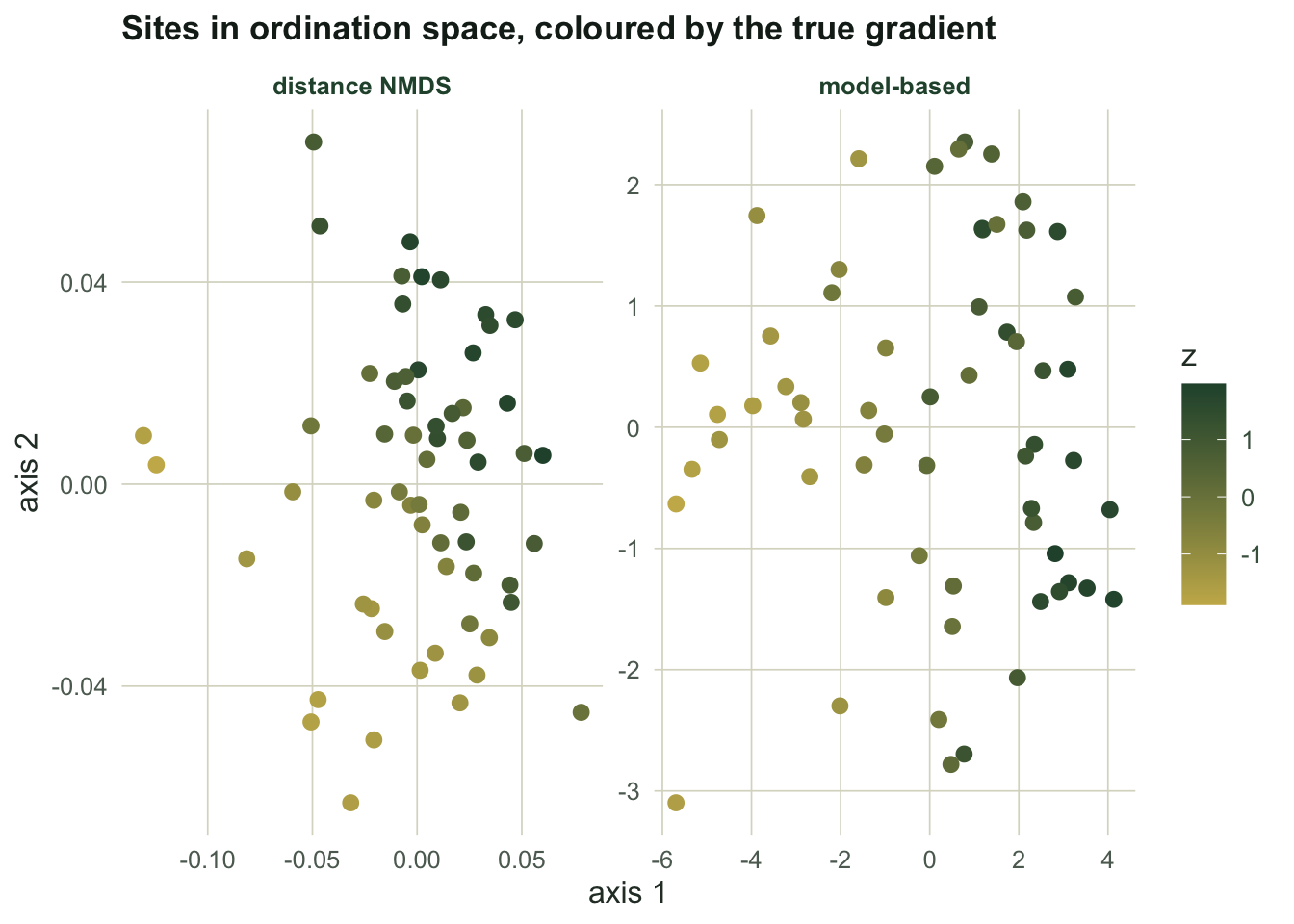
#| fig-alt: "Two ordination plots of sites, coloured by the true gradient; the model-based panel shows a clean colour sweep across an axis, the distance-based panel shows a looser diagonal sweep, gold sites at the bottom and far left and dark sites towards the top, running more along axis 2 than axis 1."
#| fig-cap: "Sites coloured by the true gradient. A clean sweep means the gradient sits on an axis."
op <- rbind(data.frame(a1 = mb1s, a2 = scale(mb2, scale = FALSE)[,1], z = z, panel = "model-based"),
data.frame(a1 = db1s, a2 = db2, z = z, panel = "distance NMDS"))
ggplot(op, aes(a1, a2, colour = z)) + geom_point(size = 2.4) +
facet_wrap(~panel, scales = "free") +
scale_colour_gradient(low = te_gold, high = te_green) +
labs(title = "Sites in ordination space, coloured by the true gradient",
x = "axis 1", y = "axis 2") + theme_te()
```
Note that the NMDS fit is not broken in its own terms: its stress is `r round(mds_stress, 3)`, in the band conventionally read as usable rather than good, where the broad layout can be believed but the fine detail cannot. It preserved the broad rank order of the dissimilarities. Low stress is a statement about the fit to the dissimilarities, not about ecology.
## Honest limits
The model-based ordination is not free of assumptions, it simply makes them explicit. It assumes a negative binomial mean-variance relationship; if that is wrong the residuals are wrong and the axes drift, which is exactly what the residual diagnostics in the companion post are for. The latent axes are identified only up to rotation and sign, so the numbers on them mean nothing absolute and two runs can look mirrored. Whether to soak up total abundance with a site term is itself a modelling choice: if differences in total abundance are the ecology, removing them is the wrong move. And an ordination of any kind is a description of pattern, not a test of cause. An NMDS axis can be a sampling-intensity axis wearing an ecological label: here the first NMDS axis tracked total abundance and the gradient sat on a diagonal of the NMDS plane, while absorbing total abundance with a site term and putting species on a common residual scale brought it onto the first axis.
## References
Hui FKC, Taskinen S, Pledger S, Foster SD, Warton DI 2015. Methods in Ecology and Evolution 6:399-411 (10.1111/2041-210X.12236).
Warton DI, Blanchet FG, O'Hara RB, Ovaskainen O, Taskinen S, Walker SC, Hui FKC 2015. Trends in Ecology and Evolution 30:766-779 (10.1016/j.tree.2015.09.007).
Dunn PK, Smyth GK 1996. Journal of Computational and Graphical Statistics 5:236-244 (10.1080/10618600.1996.10474708).
Minchin PR 1987. Vegetatio 69:89-107 (10.1007/BF00038690).
Kruskal JB 1964. Psychometrika 29:1-27 (10.1007/BF02289565).
Legendre P, Legendre L 2012. Numerical Ecology, 3rd edition. Elsevier. ISBN 978-0-444-53868-0.
## Related tutorials
- [Model-based multivariate abundance](../model-based-multivariate-abundance/)
- [Fourth-corner trait-environment analysis](../fourth-corner-trait-environment/)
- [Checking a model-based multivariate model](../checking-a-model-based-multivariate-model/)
- [Common PERMANOVA mistakes](../common-permanova-mistakes/)