Checking a model-based multivariate model

A community-level test rests on two assumptions: the right mean-variance relationship, and resampling that keeps species correlated. Here is how to check both, and what breaks when they fail.

The three posts before this one built a community-level test, a model-based ordination, and a fourth-corner test, all resting on the same two ideas. Fit a generalised linear model to each species so that abundance and variance are handled properly, and get the community answer by resampling whole sites so that species stay correlated. Both ideas are assumptions, and both can be wrong. This post is the diagnostic companion: it checks the mean-variance assumption with residuals, checks what happens to the test when either assumption fails, and marks the line past which the method stops answering the question you asked.

A community where nothing is going on

To check a test you need a case with a known answer. We simulate 50 sites and 12 species with no group difference at all, so any rejection is a false positive. Two features make it a fair test of the assumptions: the counts are overdispersed, and the species share a site-level factor, so they are positively correlated rather than independent.

gen_null <- function(seed, n = 50, S = 12, theta = 2, sd_f = 0.7) {
  set.seed(seed)
  b0 <- log(c(rep(8,4), rep(3,4), rep(1,4)))
  f  <- rnorm(n, 0, sd_f)                          # shared site factor => species correlate
  load <- runif(S, 0.5, 1.2)
  mu <- exp(outer(rep(1,n), b0) + outer(f, load))
  L  <- matrix(rnbinom(n*S, mu = as.vector(mu), size = theta), n, S)
  list(L = L, grp = rep(c("A","B"), length.out = n))   # random groups, null is true
}
d0 <- gen_null(1)
cc <- cor(log1p(d0$L))
mean_cor <- mean(cc[lower.tri(cc)])
round(mean_cor, 2)

[1] 0.23

The average between-species correlation is 0.23, positive and far from the independence a naive test assumes.

Checking the mean-variance assumption with residuals

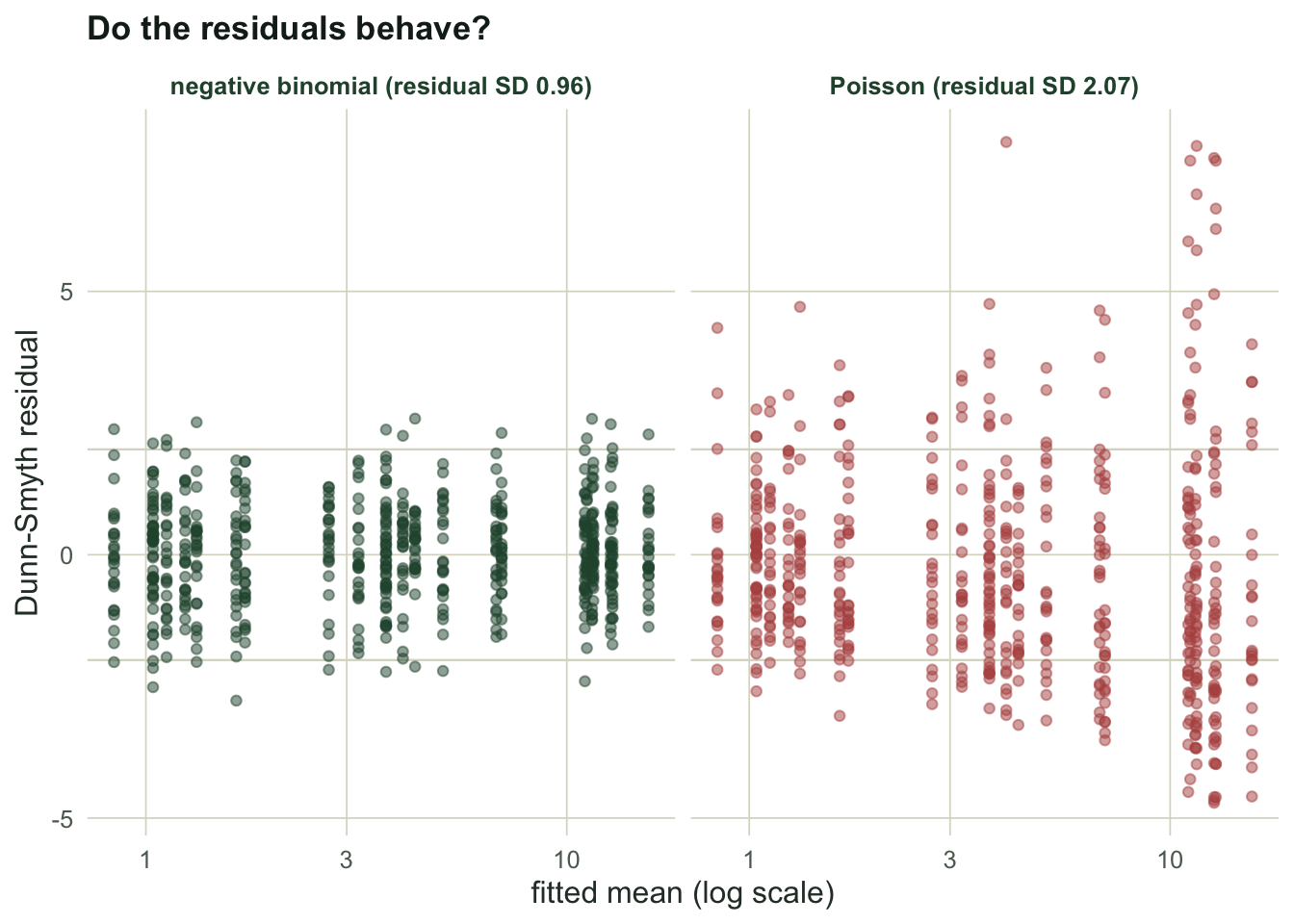
The right first move is a residual plot. Dunn-Smyth residuals turn each count into a value that should look standard normal if the model fits: take the fitted cumulative probability at the count, jitter it across its probability mass, and push it through the normal quantile function. If the model has the mean-variance relationship right, these residuals sit in a flat band with a standard deviation near one. If it does not, they fan out.

ds_pois <- function(y, mu, u) { a <- ppois(y-1, mu); b <- ppois(y, mu); qnorm(a + u*(b-a)) }
ds_nb   <- function(y, mu, th, u) {
  a <- pnbinom(y-1, mu = mu, size = th); b <- pnbinom(y, mu = mu, size = th); qnorm(a + u*(b-a)) }
mom_theta <- function(y) { m <- mean(y); v <- var(y); if (v > m*1.05) m^2/(v - m) else 1e4 }

dd <- gen_null(7); Sd <- ncol(dd$L)
fitmu <- sapply(1:Sd, function(j) ave(dd$L[,j], dd$grp, FUN = mean))   # group-mean fitted
th_j  <- apply(dd$L, 2, mom_theta)
set.seed(21); U <- matrix(runif(length(dd$L)), nrow(dd$L), Sd)
rp <- as.vector(mapply(function(j) ds_pois(dd$L[,j], fitmu[,j], U[,j]), 1:Sd))
rn <- as.vector(mapply(function(j) ds_nb(dd$L[,j], fitmu[,j], th_j[j], U[,j]), 1:Sd))
sd_rp <- sd(rp[is.finite(rp)]); sd_rn <- sd(rn[is.finite(rn)])
c(poisson_resid_sd = round(sd_rp, 2), nb_resid_sd = round(sd_rn, 2))

poisson_resid_sd      nb_resid_sd 
            2.07             0.96 

Figure 1: Dunn-Smyth residuals against fitted mean. A flat band of width about two means the model fits; the Poisson fan is overdispersion.

The Poisson residuals have a standard deviation of 2.07, twice what a good fit gives, and they spread wider as the fitted mean grows: the fingerprint of variance rising faster than the mean. The negative binomial residuals sit at 0.96, inside the band. The plot has already told us the Poisson model is the wrong one before we run a single test.

What the wrong choice costs

Now the consequence. We run the community test three ways on many null datasets. The honest version fits a negative binomial to each species, sums the likelihood-ratio statistics, and gets its p-value by permuting the group labels, which keeps whole sites intact and so preserves the correlation. Two shortcuts tempt people: keep the negative binomial but read the sum against a chi-square distribution, which assumes the species are independent; or drop back to Poisson and do the same.

nb_lr <- function(y, grp, theta) {
  mu0 <- mean(y); ll0 <- sum(dnbinom(y, mu = mu0, size = theta, log = TRUE))
  mu1 <- ave(y, grp, FUN = mean); ll1 <- sum(dnbinom(y, mu = mu1, size = theta, log = TRUE))
  2*(ll1 - ll0)
}
pois_lr <- function(y, grp) {
  mu0 <- mean(y); ll0 <- sum(dpois(y, mu0, log = TRUE))
  mu1 <- ave(y, grp, FUN = mean); ll1 <- sum(dpois(y, mu1, log = TRUE))
  2*(ll1 - ll0)
}
community <- function(L, grp, B = 149, seed = 1) {
  S <- ncol(L); th <- apply(L, 2, mom_theta)
  obs_nb <- sum(sapply(1:S, function(j) nb_lr(L[,j], grp, th[j])))
  obs_po <- sum(sapply(1:S, function(j) pois_lr(L[,j], grp)))
  set.seed(seed)
  perm <- replicate(B, { g <- sample(grp); sum(sapply(1:S, function(j) nb_lr(L[,j], g, th[j]))) })
  c(nb_perm  = (1 + sum(perm >= obs_nb)) / (B + 1),
    nb_chisq = pchisq(obs_nb, df = S, lower.tail = FALSE),
    po_chisq = pchisq(obs_po, df = S, lower.tail = FALSE))
}

M <- 240; B <- 149
res <- t(sapply(1:M, function(m) community(gen_null(2000 + m)$L, gen_null(2000 + m)$grp, B = B, seed = m)))
rate <- colMeans(res < 0.05)
round(rate, 3)

 nb_perm nb_chisq po_chisq 
   0.038    0.100    0.967 

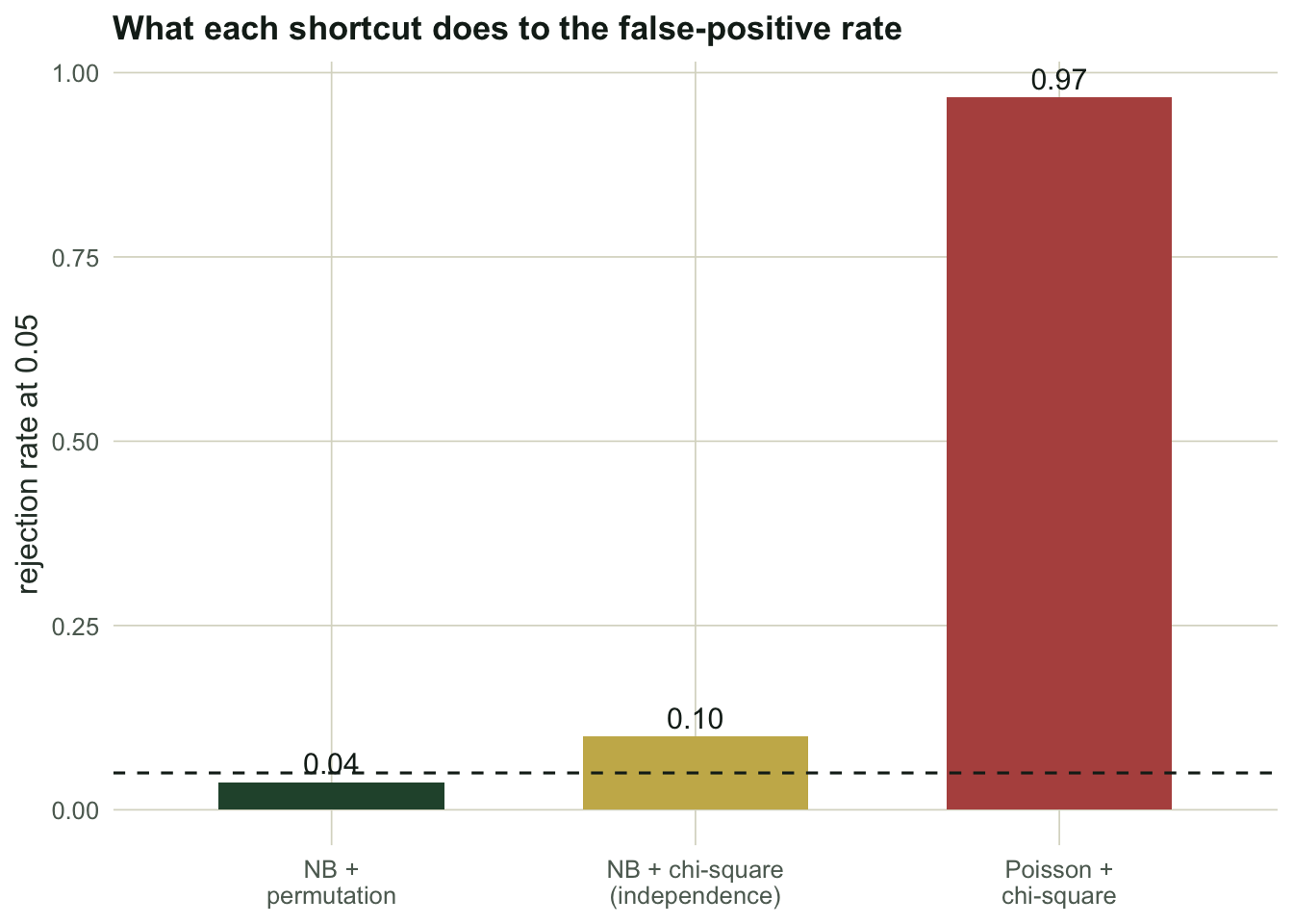
Figure 2: Rejection rate under a null with correlated, overdispersed counts. Only the permutation controls at 0.05.

The permutation test rejects a true null 0.04 of the time, on target. Keeping the negative binomial but trusting the chi-square pushes that to 0.10, because correlated species make the summed statistic more variable than a chi-square expects, so the tail is fatter than the table says. Dropping to Poisson is a disaster: 0.97, almost always significant, because the underestimated variance inflates every species’ contribution. Fixing the mean-variance relationship closes most of the gap; only resampling whole sites closes the rest.

Honest limits

A clean community test answers one question and no more: the assemblage as a whole responds to the grouping. It does not say which species drive it. The per-species statistics that fall out along the way are the raw material for that question, but they are a family of tests on correlated data and need false-discovery control before any of them earns a claim, which is a separate step. The test is also silent on why: a model-based analysis of observational counts describes association, and turning that into cause needs a design that intervenes, not a better likelihood. The permutation itself leans on exchangeability of sites under the null, so clustered or repeated-measures sampling needs a permutation scheme that respects the blocks. And a residual plot catches the mean-variance problems it was built for, not every way a model can be wrong. Within those limits the pattern across all four posts is the same one worth keeping: the model earns its answer only when its assumptions are checked, and the quiet failures, an overdispersed count fit as Poisson, correlated species treated as independent, are the ones that turn a null into a discovery.

References

Warton DI, Wright ST, Wang Y 2012. Distance-based multivariate analyses confound location and dispersion effects. Methods in Ecology and Evolution 3:89-101 (10.1111/j.2041-210X.2011.00127.x).

Wang Y, Naumann U, Wright ST, Warton DI 2012. mvabund: an R package for model-based analysis of multivariate abundance data. Methods in Ecology and Evolution 3:471-474 (10.1111/j.2041-210X.2012.00190.x).

Dunn PK, Smyth GK 1996. Randomized quantile residuals. Journal of Computational and Graphical Statistics 5:236-244 (10.1080/10618600.1996.10474708).

Hui FKC, Taskinen S, Pledger S, Foster SD, Warton DI 2015. Model-based approaches to unconstrained ordination. Methods in Ecology and Evolution 6:399-411 (10.1111/2041-210X.12236).

Warton DI 2005. Many zeros does not mean zero inflation: comparing the goodness of fit of parametric models to multivariate abundance data. Environmetrics 16:275-289.

Related tutorials

• Model-based multivariate abundance
• Model-based unconstrained ordination
• Fourth-corner trait-environment analysis
• The false discovery rate and Benjamini-Hochberg