library(FD)
library(ggplot2)
library(dplyr)
library(tidyr)Functional diversity in R with the FD package
R
functional diversity
traits
diversity
Beyond counting species: measuring functional diversity in R from mixed traits with the FD package. Gower distance, functional richness, evenness, divergence, dispersion, Rao’s quadratic entropy, and community-weighted means, with a worked redundancy contrast. A trait-based ecology tutorial.
Species richness counts the species in a community and stops there, treating a community of ten near-identical grasses as exactly as diverse as ten species spanning trees, shrubs, herbs, and nitrogen-fixers. For most questions about how a community works, that is the wrong currency. What an ecosystem does, how it captures light, cycles nutrients, resists invasion, depends on the traits its species carry, and two assemblages with the same richness can hold wildly different ranges of trait values. Functional diversity puts a number on that range.
This post measures it in R with the FD package. We build a small set of species described by mixed traits, some continuous and some categorical, collapse them into a single distance with Gower’s coefficient, and then compute the standard functional-diversity indices with dbFD: functional richness, evenness, divergence, dispersion, and Rao’s quadratic entropy, plus the community-weighted trait means. The whole point is made by a deliberate contrast: a species-rich community that is functionally redundant against a species-poor one that is functionally spread. Where the diversity indices post measured diversity from abundances alone, this one brings the traits in.
Species, traits, and three communities
We describe fifteen plant species with five traits. Three are continuous, specific leaf area (SLA), height, and seed mass, and two are categorical, growth form and whether the species fixes nitrogen. Ten of the species are a tight cluster of common herbs, similar in every trait; the other five sit at the extremes of the trait space, a small grass, a big-seeded shrub, a tall tree, a nitrogen-fixing shrub, and a tiny herb.
set.seed(77)
herbs <- data.frame(
  sla    = rnorm(10, 20, 3),
  height = rnorm(10, 0.30, 0.06),
  seed   = rnorm(10, 1.2, 0.4),
  form   = "herb", nfix = "no"
)
herbs$height <- pmax(herbs$height, 0.1); herbs$seed <- pmax(herbs$seed, 0.2)

extremes <- data.frame(
  sla    = c(16,   7,   7,  15,  30),
  height = c(0.6,  3,  22,   2, 0.15),
  seed   = c(0.3, 400, 250, 30, 0.1),
  form   = c("grass","shrub","tree","shrub","herb"),
  nfix   = c("no","no","no","yes","no")
)
traits <- rbind(herbs, extremes)
traits$form <- factor(traits$form); traits$nfix <- factor(traits$nfix)
rownames(traits) <- sprintf("sp%02d", 1:15)

c(species = nrow(traits), traits = ncol(traits),
  SLA_lo = round(min(traits$sla),0), SLA_hi = round(max(traits$sla),0))
species traits SLA_lo SLA_hi
15 5 7 30 The three communities are built to separate two ideas. Redundant holds ten of the clustered herbs: high richness, but everyone is functionally alike. Diverse holds the five extreme species: low richness, but they fill the trait space. Clumped holds the same five species as Diverse, with one of them made overwhelmingly dominant in abundance. The first pair isolates richness against functional spread; the second pair isolates the effect of abundance while the species, and therefore the trait space, stay fixed.
comm <- matrix(0, nrow = 3, ncol = 15,
               dimnames = list(c("Redundant","Diverse","Clumped"),
                               rownames(traits)))
comm["Redundant", 1:10] <- c(8,7,9,6,8,7,10,6,7,8)
ext <- sprintf("sp%02d", 11:15)
comm["Diverse", ext]    <- c(6,5,6,5,6)
comm["Clumped", ext]    <- c(40,3,3,3,3)

rowSums(comm > 0)   # species richness per community
Redundant Diverse Clumped
10 5 5 Redundant has twice the species of the other two. If richness were the whole story, it would be the most diverse community by a wide margin. It is about to come last on every measure that looks at traits.
One distance for mixed traits: Gower
Functional-diversity indices need a single distance between every pair of species, but our traits mix types: SLA is a number, growth form is a category. Gower’s coefficient (Gower 1971) handles this by computing a per-trait distance appropriate to each trait, scaling continuous traits to their range and scoring categorical traits as match or mismatch, then averaging across traits. One detail matters first: height and seed mass span orders of magnitude, from a 15 cm herb to a 22 m tree, from a 0.1 mg seed to a 400 mg one. Left raw, the giants would dominate the range-scaling and crush all variation among the smaller species, so we log-transform both before computing the distance, the routine move for traits that vary multiplicatively.
traits_an <- traits
traits_an$height <- log10(traits_an$height)
traits_an$seed   <- log10(traits_an$seed)

gd <- gowdis(traits_an)
c(min = round(min(gd),3), max = round(max(gd),3), mean = round(mean(gd),3))
min max mean
0.014 0.781 0.288 The distances run from near zero, the herb-to-herb pairs, up to about 0.78 for the most dissimilar species. That spread is the raw material every index below is built from.
The index family with dbFD
dbFD takes the trait matrix and the community matrix and returns the whole standard family of indices in one call. It ordinates the Gower distances into a trait space with a principal coordinates analysis (the same PCoA idea behind distance-based ordination), applying a Cailliez correction so the space is properly Euclidean, then computes each index in that space. We standardise functional richness to a 0-to-1 scale, the fraction of the global trait-space volume a community fills, and compute the community-weighted means on the original trait scale so they stay readable.
fd <- dbFD(traits_an, comm, corr = "cailliez", stand.FRic = TRUE,
           calc.FRic = TRUE, calc.FDiv = TRUE, calc.CWM = FALSE,
           messages = FALSE)
cwm <- functcomp(traits, comm)   # community-weighted means, raw scale

data.frame(
  community = rownames(comm), nbsp = fd$nbsp,
  FRic = round(fd$FRic, 3), FEve = round(fd$FEve, 3),
  FDiv = round(fd$FDiv, 3), FDis = round(fd$FDis, 3),
  RaoQ = round(fd$RaoQ, 3), row.names = NULL
)
community nbsp FRic FEve FDiv FDis RaoQ
1 Redundant 10 0.000 0.942 0.808 0.035 0.001
2 Diverse 5 0.578 0.905 0.848 0.361 0.137
3 Clumped 5 0.578 0.548 0.737 0.171 0.056Five indices, each a different facet. FRic (functional richness) is the volume of trait space the species enclose, a convex hull (Villeger et al. 2008). FEve (functional evenness) measures how regularly abundance is spread through that space. FDiv (functional divergence) measures how far abundance sits from the centre, toward the edges. FDis (functional dispersion) is the abundance-weighted mean distance of species to their centroid (Laliberte & Legendre 2010). RaoQ is Rao’s quadratic entropy, the abundance-weighted mean distance between all species pairs (Botta-Dukat 2005). The first reads only which species are present; the rest also read how abundant each is.
Richness is not functional diversity
The headline contrast is in the first two rows. Redundant has ten species and Diverse has five, yet Diverse fills 58% of the trait space while Redundant fills essentially none of it, and Diverse’s functional dispersion is roughly ten times larger. Twice the richness, a fraction of the functional diversity. Plotting the trait space shows why immediately.
te_paper <- "#f5f4ee"; te_ink <- "#16241d"; te_body <- "#2c3a31"; te_line <- "#dad9ca"
base_theme <- theme_minimal(base_size = 12) +
  theme(panel.grid.minor = element_blank(),
        panel.grid.major = element_line(color = te_line, linewidth = 0.3),
        plot.background  = element_rect(fill = te_paper, color = NA),
        panel.background = element_rect(fill = te_paper, color = NA),
        axis.text = element_text(color = te_body), axis.title = element_text(color = te_ink),
        plot.title = element_text(color = te_ink, face = "bold", size = 12),
        legend.title = element_text(color = te_ink, size = 9),
        legend.text = element_text(color = te_body, size = 8))

pco <- ade4::dudi.pco(ade4::cailliez(gd), scannf = FALSE, nf = 2)
ax  <- pco$li; colnames(ax) <- c("A1","A2"); ax$species <- rownames(traits)
sel <- c("Redundant","Diverse")
hull_df <- do.call(rbind, lapply(sel, function(cm){
  sp <- colnames(comm)[comm[cm,] > 0]; sub <- ax[ax$species %in% sp, c("A1","A2")]
  data.frame(sub[chull(sub$A1, sub$A2), ], community = cm)
}))
pt_df <- do.call(rbind, lapply(sel, function(cm){
  sp <- colnames(comm)[comm[cm,] > 0]
  data.frame(ax[ax$species %in% sp, c("A1","A2")], community = cm)
}))
cols3 <- c("Redundant"="#b5534e","Diverse"="#2f8f63","Clumped"="#c9a227")

ggplot() +
  geom_polygon(data = hull_df, aes(A1, A2, fill = community, color = community),
               alpha = 0.18, linewidth = 0.8) +
  geom_point(data = pt_df, aes(A1, A2, color = community), size = 2.6) +
  scale_fill_manual(values = cols3, name = NULL) +
  scale_color_manual(values = cols3, name = NULL) +
  labs(x = "PCoA axis 1", y = "PCoA axis 2",
       title = "Trait space: ten clustered species, five spread ones") +
  base_theme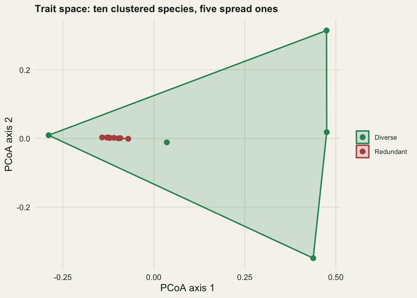
The ten redundant species (in red) sit almost on top of one another in a near-flat line: they differ along essentially one direction, SLA, and nothing else, so the area they enclose is negligible. The five diverse species (in green) reach into the corners and wrap a large triangle around the whole space. This also exposes a real limitation of FRic worth knowing before you trust it. Functional richness is a hull volume, and a set of points strung along a single axis encloses no volume no matter how many points there are; that is why Redundant’s FRic collapses to effectively zero. FRic also needs more species than retained trait dimensions to be computable at all, and it is sensitive to outlying species. Dispersion-based measures like FDis and RaoQ degrade more gracefully in exactly these situations, which is part of why Laliberte & Legendre (2010) introduced FDis. The more reliable reading of the contrast is the dispersion one: 0.035 against 0.361.
There is a deeper point here than a quirk of one index. Botta-Dukat (2005) noted that adding a species to a community can lower its functional diversity, because a new species raises abundance-based diversity but may sit close to species already present and so drag down the average dissimilarity. Richness and functional diversity are not two names for the same thing, and they can move in opposite directions.
Abundance changes the answer, for most of the indices
The second contrast holds the species fixed and changes only the abundances. Diverse and Clumped contain the identical five extreme species, so their trait space, and their functional richness, are exactly the same. Everything that reads abundance, though, moves sharply.
res <- data.frame(
  community = rownames(comm),
  FRic = fd$FRic, FEve = fd$FEve, FDiv = fd$FDiv, FDis = fd$FDis, RaoQ = fd$RaoQ
)
ind_long <- res |>
  pivot_longer(-community, names_to = "index", values_to = "value") |>
  mutate(community = factor(community, levels = c("Redundant","Diverse","Clumped")),
         index = factor(index, levels = c("FRic","FEve","FDiv","FDis","RaoQ")))

ggplot(ind_long, aes(community, value, fill = community)) +
  geom_col(width = 0.7) +
  facet_wrap(~ index, scales = "free_y", nrow = 1) +
  scale_fill_manual(values = cols3, guide = "none") +
  labs(x = NULL, y = NULL,
       title = "Functional diversity indices across the three communities") +
  base_theme +
  theme(axis.text.x = element_text(angle = 35, hjust = 1, size = 8),
        strip.text = element_text(color = te_ink, face = "bold"))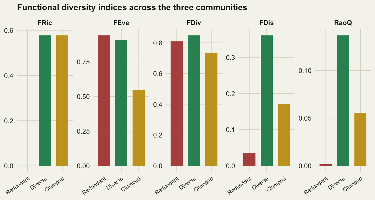
The FRic panel shows Diverse and Clumped at the same height, as they must, since the species are identical. But making one species dominate collapses functional evenness from about 0.91 to 0.55, pulls functional divergence down, halves functional dispersion, and more than halves Rao’s quadratic entropy. The community still spans the same trait space; it just now sits almost entirely in one corner of it. Notice too that Redundant scores high on evenness, higher than Diverse, because its ten species carry roughly equal abundances. Evenness and dispersion are answering different questions, and a community can be even while being functionally dispersed by almost nothing.
Community-weighted means: the average phenotype
The indices above describe the spread of traits. The community-weighted mean describes their centre, the abundance-weighted average trait value, and it is often what links functional composition to ecosystem processes. It also reads naturally as the community’s typical phenotype.
cwm sla height seed form nfix
Redundant 21.05132 0.3086458 1.282473 herb no
Diverse 15.28571 5.7678571 130.442857 shrub no
Clumped 15.71154 2.0278846 39.467308 grass noThe functional identities are distinct. Redundant is a community of small, fast herbs: high SLA, a few centimetres tall, tiny seeds. Diverse is pulled toward the woody extremes, with a much taller, larger-seeded average and a shrub as its modal growth form. Clumped, dominated by its grass, takes on that grass’s signature. Two communities can share a trait space yet have very different centres of mass, and the CWM is what records it.
Which index, and the caveats that travel with them
There is no single best functional-diversity index; the family exists because the facets are genuinely different. Use FRic when the question is about the range of strategies present, but respect its requirements: more species than dimensions, and a wariness of near-collinear or outlier-driven cases where the hull misbehaves. Use FDis or Rao’s Q for an abundance-aware measure of overall functional spread that stays well-behaved with few species. Use FEve and FDiv when how abundance is distributed through trait space is the point. Use the CWM when functional identity, the average trait, matters more than its spread.
Two choices upstream shape all of them. Trait selection is the first: the indices only know about the traits you feed them, so a community that is diverse in traits you left out will look redundant. Trait scaling is the second, as the log-transform of height and seed mass here already showed; the Gower distance, and everything built on it, shifts when you change how traits are weighted or transformed. Functional diversity is a powerful step beyond richness, but it inherits all the judgement that goes into deciding what “functional” means. For the abundance side of diversity that these indices extend, the diversity indices post is the companion; for how communities differ from each other rather than within themselves, the beta-diversity post partitions that turnover.
Takeaways
Species richness treats species as interchangeable; functional diversity does not, and the two can diverge completely, as the redundant ten-species community here filling almost none of the trait space its five-species rival fills. Gower’s distance turns mixed continuous and categorical traits into one dissimilarity (log-transform traits that span orders of magnitude first), and dbFD returns the whole index family at once. FRic is a hull volume that reads only presence and needs enough non-collinear species to compute; FDis and Rao’s Q add abundance and stay well-behaved; FEve and FDiv describe how abundance is distributed; the CWM gives the average phenotype. Adding a species can lower functional diversity (Botta-Dukat 2005), and every index is only as meaningful as the traits and scaling you chose.
References
Botta-Dukat, Z. (2005). Rao’s quadratic entropy as a measure of functional diversity based on multiple traits. Journal of Vegetation Science, 16(5), 533-540. https://doi.org/10.1111/j.1654-1103.2005.tb02393.x
Gower, J. C. (1971). A general coefficient of similarity and some of its properties. Biometrics, 27(4), 857-871. https://doi.org/10.2307/2528823
Laliberte, E. & Legendre, P. (2010). A distance-based framework for measuring functional diversity from multiple traits. Ecology, 91(1), 299-305. https://doi.org/10.1890/08-2244.1
Mason, N. W. H., Mouillot, D., Lee, W. G. & Wilson, J. B. (2005). Functional richness, functional evenness and functional divergence: the primary components of functional diversity. Oikos, 111(1), 112-118. https://doi.org/10.1111/j.0030-1299.2005.13886.x
Villeger, S., Mason, N. W. H. & Mouillot, D. (2008). New multidimensional functional diversity indices for a multifaceted framework in functional ecology. Ecology, 89(8), 2290-2301. https://doi.org/10.1890/07-1206.1