---
title: "Community weighted means in R"
description: "The community weighted mean is the most reported trait statistic in ecology. What it measures, what it hides, and the identity linking it to the fourth corner."
date: "2026-06-17 09:00"
date-modified: "2026-10-14"
categories: [R, traits, functional ecology, community ecology, ecology tutorial]
image: thumbnail.png
image-alt: "A scatter plot of community weighted mean specific leaf area rising along a moisture gradient, annotated with the two different correlations the same data give."
---
*Corrected 14 October 2026: the subtitle of the figure of eighty data sets said the gap to the diagonal is the trait variation the plots do not separate, which reads the difference between the two correlations as a variance share; it now says the fourth corner is the weighted CWM correlation times the square root of the between-plot share.*
*Corrected 1 October 2026: the closing advice said the between-plot share of trait variance is the discount factor and the difference between the two correlations; its square root is that factor, and the factor is their ratio. The post also now says that the exact relation holds for the CWM correlation weighted by plot totals, and no longer calls rare wet end specialists the ordinary state of affairs in a real flora.*
Almost every trait paper contains the same three lines of code: take a site by species table, take a trait value per species, average the trait over the species present, weighting by abundance. The result is the community weighted mean, and it gets regressed against whatever environmental variable is to hand.
The statistic is easy. The trouble is that it is a mean, and a mean is a summary of a distribution you then stop looking at. This post builds a CWM from scratch, measures what it throws away, shows the exact identity that links it to the fourth corner statistic, and prices the trait coverage rule that everyone quotes and nobody checks.
## A gradient, thirty-six species, one trait
Forty plots along a moisture gradient. Each of thirty-six species has an optimum on the gradient, a Gaussian response curve around it, and a specific leaf area (SLA) that increases with its optimum: species from the wet end are the soft, fast, high SLA ones. Abundances are Poisson counts.
```{r data}
set.seed(308)
n_site <- 40; n_sp <- 36
moist <- seq(0, 1, length.out = n_site)
opt   <- runif(n_sp, -0.10, 1.10)              # species optima on the gradient
sla   <- 10 + 18 * opt + rnorm(n_sp, 0, 2.2)   # the trait: tied to the optimum
amax  <- rlnorm(n_sp, log(28), 0.40)           # how common each species is
mu <- outer(moist, opt, function(e, o) exp(-(e - o)^2 / (2 * 0.18^2)))
L  <- matrix(rpois(n_site * n_sp, sweep(mu, 2, amax, "*")), n_site, n_sp)
dim(L); sum(L); range(rowSums(L > 0))
```
The CWM is one line. Weighted by abundance, and for comparison weighted by presence alone:
```{r cwm}
cwm <- function(A, t) as.vector(A %*% t / rowSums(A))
cwm_ab <- cwm(L, sla)
cwm_pa <- cwm((L > 0) * 1, sla)
fit <- lm(cwm_ab ~ moist)
round(coef(summary(fit)), 3)
```
```{r fig-gradient}
#| echo: false
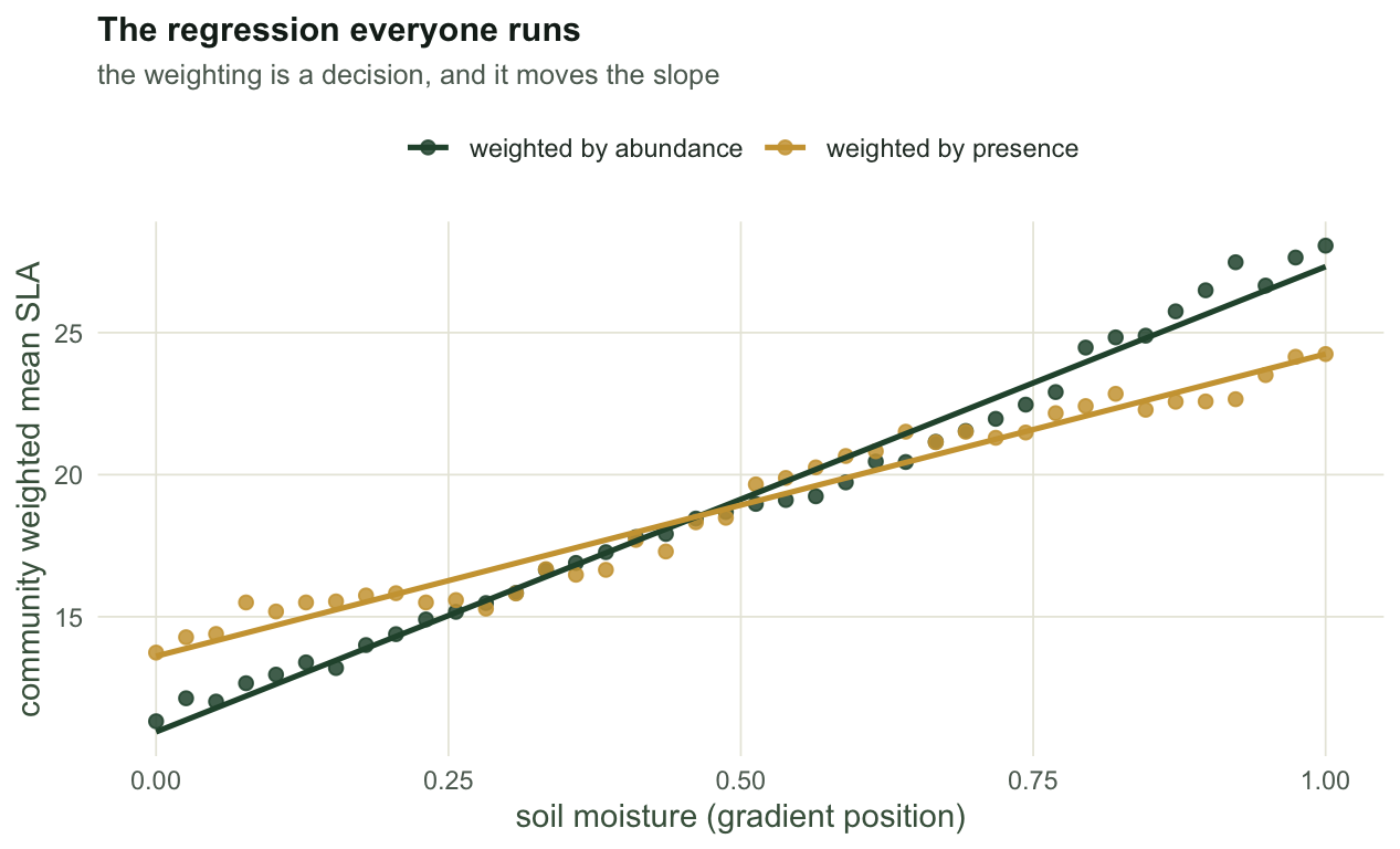
#| fig-cap: "Community weighted mean SLA along the moisture gradient. Weighting by abundance and weighting by presence give the same story with different slopes: the presence version lets a single stem count as much as a dominant."
#| fig-alt: "Scatter plot with moisture on the x axis and community weighted mean SLA on the y axis. Two sets of points with fitted lines both rise from left to right; the abundance weighted line is steeper than the presence weighted line."
#| fig-width: 6.6
#| fig-height: 4.0
suppressMessages(library(ggplot2))
theme_te <- theme_minimal(base_size = 11) +
theme(
plot.background = element_rect(fill = "#f5f4ee", colour = NA),
panel.background = element_rect(fill = "#f5f4ee", colour = NA),
panel.grid.minor = element_blank(),
panel.grid.major = element_line(colour = "#e8e7dc", linewidth = 0.3),
axis.title = element_text(colour = "#46604a"),
axis.text = element_text(colour = "#5d6b61"),
plot.title = element_text(colour = "#16241d", face = "bold", size = 11.5),
plot.subtitle = element_text(colour = "#5d6b61", size = 9.5),
legend.position = "top", legend.title = element_blank(),
legend.text = element_text(colour = "#2c3a31"))
gd <- data.frame(moist = rep(moist, 2), cwm = c(cwm_ab, cwm_pa),
w = rep(c("weighted by abundance", "weighted by presence"), each = n_site))
ggplot(gd, aes(moist, cwm, colour = w)) +
geom_point(size = 1.9, alpha = 0.85) +
geom_smooth(method = "lm", formula = y ~ x, se = FALSE, linewidth = 0.9) +
scale_colour_manual(values = c("weighted by abundance" = "#275139",
"weighted by presence" = "#cda23f")) +
labs(x = "soil moisture (gradient position)", y = "community weighted mean SLA",
title = "The regression everyone runs",
subtitle = "the weighting is a decision, and it moves the slope") +
theme_te
```
Two lines, two slopes, one gradient. The weighting choice is not a detail: presence weighting asks what the species list says, abundance weighting asks what the biomass says, and they are different questions about the same plot.
## One number, many communities
The CWM is a mean, so it is blind in the way every mean is blind. Two plots with the same species richness, the same total abundance and the same CWM:
```{r hidden}
comm <- rbind(A = c(25, 25, 25, 25), B = c(25, 25, 25, 25))
tr_A <- c(18, 19, 21, 22)          # four species with similar leaves
tr_B <- c(8, 9, 31, 32)            # two tough species and two soft ones
cwv  <- function(a, t) sum(a * (t - sum(a * t) / sum(a))^2) / sum(a)
c(CWM_A = sum(comm["A", ] * tr_A) / 100, CWM_B = sum(comm["B", ] * tr_B) / 100,
  sd_A  = sqrt(cwv(comm["A", ], tr_A)),  sd_B = sqrt(cwv(comm["B", ], tr_B)))
```
Same centre, one community packed into four SLA units and the other spread over twenty-four. If your hypothesis is about filtering towards a trait optimum, the CWM is the right statistic. If it is about limiting similarity, niche packing or functional insurance, the CWM cannot see your hypothesis at all: you want the spread, and that is what [functional diversity indices](../functional-diversity-fd/) are for.
In the simulated gradient the same blindness is quieter but real. The weighted variance of SLA within a plot averages:
```{r cwvsim}
cwv_site <- vapply(seq_len(n_site), function(i) cwv(L[i, ], sla), 0)
round(c(mean_within_sd = mean(sqrt(cwv_site)),
        sd_of_cwm = sd(cwm_ab), total_sd = sd(rep(sla, colSums(L)))), 2)
```
Nearly as much SLA variation sits inside an average plot (`r sprintf("%.1f", mean(sqrt(cwv_site)))` units) as separates the plot means along the entire gradient (`r sprintf("%.1f", sd(cwm_ab))` units). The regression in the figure above is a real signal computed on one side of a roughly even split. The exact split is the subject of the next section.
## The fourth corner is a rescaled CWM correlation
The other way to link traits and environment is the [fourth corner statistic](../fourth-corner-trait-environment/): correlate the environmental value and the trait value across the inflated table, where every individual contributes one row of (environment at its plot, trait of its species). Build it literally, one row per individual:
```{r inflated}
ii <- rep(seq_len(n_site), times = rowSums(L))
jj <- unlist(lapply(seq_len(n_site), function(i) rep(seq_len(n_sp), times = L[i, ])))
length(ii)                                   # one row per individual
r_inf <- cor(moist[ii], sla[jj])
r_inf
```
That is a correlation over `r format(length(ii), big.mark = ",")` rows, and it is `r sprintf("%.3f", r_inf)`. The CWM correlation, over forty rows, is a different number:
```{r cwmcor}
c(cwm_correlation = cor(cwm_ab, moist), fourth_corner = r_inf)
```
Both are correct. Once the CWM correlation is weighted by plot totals, which barely changes it here, they are the same covariance divided by different things, and the relation between them is exact. Work the weighted algebra: let `p_ij` be the abundance share of species j at site i, `w_i` the row share, `c_j` the column share.
```{r identity}
P  <- L / sum(L); w <- rowSums(P); cj <- colSums(P)
eb <- sum(w * moist);  Ve <- sum(w * (moist - eb)^2)      # weighted by site total
tb <- sum(cj * sla);   Vt <- sum(cj * (sla - tb)^2)       # weighted by species total
Vc <- sum(w * (cwm_ab - tb)^2)                            # variance of the CWM values
Vwithin <- sum(vapply(seq_len(n_site), function(i) sum(P[i, ] * (sla - cwm_ab[i])^2), 0))
cov_w <- sum(w * (moist - eb) * (cwm_ab - tb))
r_fc  <- cov_w / sqrt(Ve * Vt)
r_cwm <- cov_w / sqrt(Ve * Vc)
shrink <- sqrt(Vc / Vt)
c(inflated = r_inf, weighted_formula = r_fc, gap = abs(r_inf - r_fc))
```
The forty by thirty-six weighted formula reproduces the fifteen-thousand-row correlation to within floating-point rounding. The numerator is identical in both statistics, because summing the trait over each row is exactly what the CWM does:
```{r split}
c(Vt = Vt, Vc = Vc, Vwithin = Vwithin, gap = abs(Vt - Vc - Vwithin))
c(r_cwm = r_cwm, times_shrink = shrink, product = r_cwm * shrink,
  r_fc = r_fc, gap = abs(r_fc - r_cwm * shrink))
```
Two exact statements fall out. First, the total trait variance splits into the variance of the plot means plus the mean variance within plots: `r sprintf("%.2f", Vt)` = `r sprintf("%.2f", Vc)` + `r sprintf("%.2f", Vwithin)`, exact up to floating-point rounding. Second, and this is the useful one:
```
r_fourth_corner = r_CWM * sqrt( variance of the plot means / total trait variance )
```
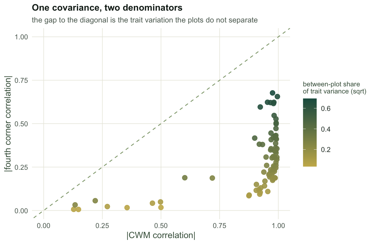
The fourth corner correlation is the weighted CWM correlation multiplied by the square root of the between-plot share of the trait variance. Here that share is `r sprintf("%.0f%%", 100 * Vc / Vt)`, so the discount factor is `r sprintf("%.3f", shrink)` and `r sprintf("%.3f", r_cwm)` becomes `r sprintf("%.3f", r_fc)`. The two numbers can never disagree about the sign, and the fourth corner is never the larger of the two in absolute value. Peres-Neto, Dray & ter Braak (2017) is the paper that spells this out.
Eighty randomly drawn designs, all sizes and gradient widths, confirm both halves:
```{r sweep}
#| cache: false
wcor_parts <- function(A, e, t) {
  P <- A / sum(A); w <- rowSums(P); cj <- colSums(P)
  eb <- sum(w * e); Ve <- sum(w * (e - eb)^2)
  tb <- sum(cj * t); Vt <- sum(cj * (t - tb)^2)
  m  <- as.vector(A %*% t / rowSums(A)); Vc <- sum(w * (m - tb)^2)
  cw <- sum(w * (e - eb) * (m - tb))
  c(r_fc = cw / sqrt(Ve * Vt), r_cwm = cw / sqrt(Ve * Vc), shrink = sqrt(Vc / Vt))
}
set.seed(3082)
sw <- as.data.frame(t(replicate(80, {
  ns <- sample(20:45, 1); nsp <- sample(15:40, 1)
  e2 <- runif(ns); op2 <- runif(nsp, -0.2, 1.2); tl <- runif(1, 0.10, 0.60)
  t2 <- rnorm(nsp, 20, 6) + runif(1, -20, 20) * op2
  m2 <- outer(e2, op2, function(a, b) exp(-(a - b)^2 / (2 * tl^2)))
  A  <- matrix(rpois(ns * nsp, sweep(m2, 2, rlnorm(nsp, log(20), 0.6), "*")), ns, nsp)
  ok <- rowSums(A) > 0; A <- A[ok, , drop = FALSE]; e2 <- e2[ok]
  kp <- colSums(A) > 0
  wcor_parts(A[, kp, drop = FALSE], e2, t2[kp])
})))
sw$gap <- abs(sw$r_fc - sw$r_cwm * sw$shrink)
c(max_gap = max(sw$gap), fc_never_larger = mean(abs(sw$r_fc) <= abs(sw$r_cwm) + 1e-12),
  shrink_min = min(sw$shrink), shrink_max = max(sw$shrink))
```
```{r fig-identity}
#| echo: false
#| fig-cap: "Eighty simulated data sets. Every point sits below the dashed one to one line: the fourth corner correlation is the weighted CWM correlation multiplied by the square root of the between-plot share of trait variance (the colour), and the identity holds to machine precision."
#| fig-alt: "Scatter plot of fourth corner correlation against CWM correlation for eighty simulated data sets. All points fall below a dashed diagonal line, coloured by a shrink factor from pale yellow at low values to dark green at high values."
#| fig-width: 6.6
#| fig-height: 4.3
ggplot(sw, aes(abs(r_cwm), abs(r_fc), colour = shrink)) +
geom_abline(slope = 1, intercept = 0, linetype = 2, colour = "#93a87f") +
geom_point(size = 2.6, alpha = 0.9) +
scale_colour_gradient(low = "#c9b458", high = "#1d5b4e",
name = "between-plot share\nof trait variance (sqrt)") +
coord_cartesian(xlim = c(0, 1), ylim = c(0, 1)) +
labs(x = "|CWM correlation|", y = "|fourth corner correlation|",
title = "One covariance, two denominators",
subtitle = "the fourth corner is the weighted CWM correlation times the square root of the between-plot share") +
theme_te + theme(legend.position = "right",
legend.title = element_text(colour = "#46604a", size = 8.5))
```
The discount is not a nuisance. It is the honest part of the statistic, and it earns its keep when the compositional turnover is weak. Draw plots from a single pool, so that no species prefers anything and the CWM values differ only by sampling noise:
```{r noturnover}
set.seed(3083)
nt <- t(replicate(400, {
  A <- matrix(rpois(30 * 25, 6), 30, 25)     # every plot from the same pool
  wcor_parts(A, runif(30), rnorm(25, 20, 5))
}))
c(mean_abs_r_cwm = mean(abs(nt[, "r_cwm"])), mean_abs_r_fc = mean(abs(nt[, "r_fc"])),
  cwm_above_0.3 = mean(abs(nt[, "r_cwm"]) > 0.30), fc_above_0.3 = mean(abs(nt[, "r_fc"]) > 0.30))
```
With nothing whatsoever going on, the CWM correlation clears 0.30 in `r sprintf("%.0f%%", 100 * mean(abs(nt[, "r_cwm"]) > 0.30))` of the runs here and the fourth corner in `r sprintf("%.0f%%", 100 * mean(abs(nt[, "r_fc"]) > 0.30))`. The first of those figures is an estimate of the null rate from a finite set of draws, not the rate itself. A correlation is scale free, and that is the problem: the CWM values here span only a small fraction of the trait range, and correlating them with anything is correlating noise with anything. The fourth corner rescaling remembers how little the plots differ. It does not fix the significance test, which is a separate and worse problem ([here is what it costs](../checking-a-trait-environment-analysis/)).
## How many species need a trait value?
Nobody measures leaves on every species. The received rule is to cover about 80% of the abundance and to stop. The rule has an exact arithmetic behind it. Split the site into the covered species and the rest, with local coverage `c_i`:
```
CWM_full[i] = c[i] * CWM_covered[i] + (1 - c[i]) * mean_trait_of_the_missing[i]
```
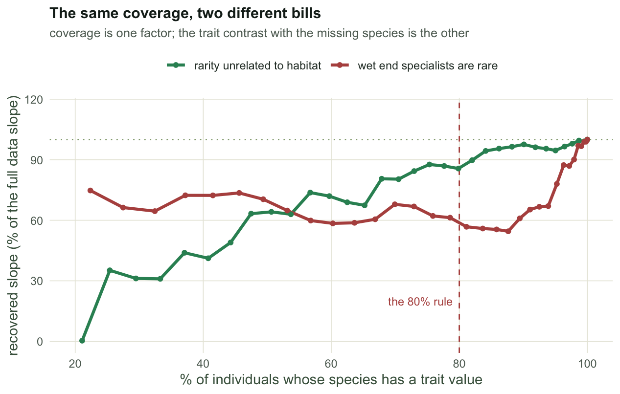
so the error you make by ignoring the missing species is exactly `(1 - c_i)` times the trait contrast between the two groups. Coverage is one factor of a product, and the rule quotes only that factor.
Two surveys, identical except for one thing. In the first, how common a species is has nothing to do with where it grows. In the second, the wet end specialists are the rare ones, as the specialists of one habitat can be in a real flora.
```{r coversim}
sim <- function(seed, rare_wet) {
  set.seed(seed)
  o <- runif(36, -0.10, 1.10)
  t <- 10 + 18 * o + rnorm(36, 0, 2.2)
  a <- rlnorm(36, log(28) - rare_wet * o, 0.40)        # rare_wet tilts abundance
  m <- outer(seq(0, 1, length.out = 40), o, function(e, x) exp(-(e - x)^2 / (2 * 0.18^2)))
  list(A = matrix(rpois(40 * 36, sweep(m, 2, a, "*")), 40, 36),
       e = seq(0, 1, length.out = 40), t = t, opt = o)
}
cover_curve <- function(s) {
  ord  <- order(colSums(s$A), decreasing = TRUE)       # measure the common ones first
  b0   <- unname(coef(lm(cwm(s$A, s$t) ~ s$e))[2])   # named coefs poison c()
  out <- t(vapply(seq_along(ord), function(k) {
    keep <- ord[seq_len(k)]; sub <- s$A[, keep, drop = FALSE]
    ok <- rowSums(sub) > 0
    b  <- unname(coef(lm(cwm(sub[ok, , drop = FALSE], s$t[keep]) ~ s$e[ok]))[2])
    c(k = k, cover = sum(colSums(s$A)[keep]) / sum(s$A), slope = b,
      worst_local = min(rowSums(sub) / rowSums(s$A)))
  }, numeric(4)))
  data.frame(out, rel = out[, "slope"] / b0, b0 = b0)
}
cc_flat <- cover_curve(sim(308, 0));  cc_tilt <- cover_curve(sim(308, 2.2))
k1 <- which(cc_flat$cover >= 0.80)[1]; k2 <- which(cc_tilt$cover >= 0.80)[1]
rbind(unrelated = c(species = k1, coverage = cc_flat$cover[k1], slope = cc_flat$slope[k1],
                    percent_of_true = 100 * cc_flat$rel[k1], worst_local = cc_flat$worst_local[k1]),
      rare_wet  = c(species = k2, coverage = cc_tilt$cover[k2], slope = cc_tilt$slope[k2],
                    percent_of_true = 100 * cc_tilt$rel[k2], worst_local = cc_tilt$worst_local[k2]))
```
```{r fig-coverage}
#| echo: false
#| fig-cap: "Recovered CWM slope against trait coverage in two surveys with the same 80% target. In the survey where the wet end specialists are the rare ones, the curve sits at 57% of the slope at the 80% mark."
#| fig-alt: "Line plot of the recovered CWM slope as a percentage of the true slope against the fraction of individuals covered by trait measurements. One curve is near full recovery by the 80% mark; the other stays far below, crossing the 80% coverage mark near 57%."
#| fig-width: 6.6
#| fig-height: 4.2
cd <- rbind(data.frame(cc_flat, case = "rarity unrelated to habitat"),
data.frame(cc_tilt, case = "wet end specialists are rare"))
cd <- subset(cd, cover >= 0.20) # below three species the slope is not defined
ggplot(cd, aes(100 * cover, 100 * rel, colour = case)) +
geom_hline(yintercept = 100, linetype = 3, colour = "#93a87f") +
geom_vline(xintercept = 80, linetype = 2, colour = "#b5534e") +
geom_line(linewidth = 1.1) + geom_point(size = 1.4) +
annotate("text", x = 79, y = 20, hjust = 1, size = 3.1, colour = "#b5534e",
label = "the 80% rule") +
scale_colour_manual(values = c("rarity unrelated to habitat" = "#2f8f63",
"wet end specialists are rare" = "#b5534e")) +
coord_cartesian(xlim = c(20, 100), ylim = c(0, 115)) +
labs(x = "% of individuals whose species has a trait value",
y = "recovered slope (% of the full data slope)",
title = "Coverage against recovered slope, two surveys",
subtitle = "coverage is one factor; the trait contrast with the missing species is the other") +
theme_te
```
At about the same coverage (`r sprintf("%.0f%%", 100 * cc_flat$cover[k1])` and `r sprintf("%.0f%%", 100 * cc_tilt$cover[k2])`), the first survey returns `r sprintf("%.0f%%", 100 * cc_flat$rel[k1])` of the slope and the second `r sprintf("%.0f%%", 100 * cc_tilt$rel[k2])`. The mechanism is in the last column of the table: overall coverage is a survey level number, the CWM is a plot level number, and the plot where the missing species live is at `r sprintf("%.0f%%", 100 * cc_tilt$worst_local[k2])` local coverage while the survey reads `r sprintf("%.0f%%", 100 * cc_tilt$cover[k2])`.
The rule is not wrong. It is incomplete in a way that its own diagnostic cannot see: you can measure the coverage, but the trait contrast with the species you did not measure is knowable only by measuring them. Report the worst local coverage, not the survey mean, and say which species you skipped.
## What to report
- The CWM, the weighting used, and the weighted standard deviation of the trait inside plots. The last one tells the reader how much of the trait variation the plot means are actually about.
- The between-plot share of the trait variance. It is one line, its square root is the discount factor above, and that factor is the ratio of the fourth corner correlation to the weighted CWM correlation.
- The worst local trait coverage, and the list of unmeasured species.
- Which averaging you used: species means from a database, or trait values measured at the plot. That choice has its own arithmetic, and it is [the next post](../intraspecific-trait-variability/).
## Where to go next
The CWM is a summary of one trait, at one place, from one table. Three directions lead out. The spread it discards is measured by [functional diversity indices](../functional-diversity-fd/). The averaging it assumes is picked apart by [the intraspecific decomposition](../intraspecific-trait-variability/). The correlation it produces has a significance test that does not work, which is the subject of [the checking post](../checking-a-trait-environment-analysis/) and, for the fourth corner side of the same coin, of [the fourth corner tutorial](../fourth-corner-trait-environment/).
## References
- Garnier, Cortez, Billes et al 2004 Ecology 85(9):2630-2637 (10.1890/03-0799)
- Lavorel, Grigulis, McIntyre et al 2008 Functional Ecology 22(1):134-147 (10.1111/j.1365-2435.2007.01339.x)
- Pakeman & Quested 2007 Applied Vegetation Science 10(1):91-96 (10.1111/j.1654-109X.2007.tb00507.x)
- Peres-Neto, Dray & ter Braak 2017 Ecography 40(7):806-816 (10.1111/ecog.02302)
- Dray & Legendre 2008 Ecology 89(12):3400-3412 (10.1890/08-0349.1)
## Related tutorials
- [The fourth corner: linking traits to the environment](../fourth-corner-trait-environment/)
- [Intraspecific trait variability in R](../intraspecific-trait-variability/)
- [Checking a functional diversity analysis](../checking-a-functional-diversity-analysis/)
- [Checking a trait environment analysis](../checking-a-trait-environment-analysis/)