---
title: "RLQ analysis in R: traits, sites and environment"
description: "RLQ on three tables from scratch in base R: the exact co-inertia decomposition, and the measured cost of maximising covariance rather than correlation."
date: "2026-06-17 12:00"
date-modified: "2026-09-30"
categories: [R, ordination, functional traits, community ecology, ecology tutorial]
image: thumbnail.png
image-alt: "One line panel with round markers, plotted against redundant environmental proxies added from 0 to 4: both series start together near 0.47, then a dark green co-inertia series climbs steadily to about 0.89 while a gold correlation series stays flat near 0.46."
---
*Corrected 30 September 2026: the post called elevation's unit-length loading its share of the axis, which made a value above one half read as a minority; it now gives the loading and its square, which is the share.*
You have three tables. Sites by environment (call it R), sites by species (L), and species by traits (Q). The question is whether the traits track the environment, and the awkward part is that no site ever meets a trait: the two tables share no dimension. Only the species table connects them.
RLQ answers this by finding the pair of directions, one through the environment and one through the traits, whose association across L is as large as possible. It is a beautiful piece of machinery and it fits in about fifteen lines of base R. It also makes one choice that nobody tells you about, and this post measures what that choice costs.
## Setup
Sixty sites along an elevation gradient, forty species. Species differ in specific leaf area, and SLA sets where on the gradient a species peaks. One decoy trait and two decoy environmental variables ride along.
```{r data}
set.seed(3110)
n_site <- 60; n_sp <- 40

elev_z <- as.numeric(scale(seq(-2, 2, length.out = n_site) + rnorm(n_site, 0, 0.25)))
sla_z  <- as.numeric(scale(rnorm(n_sp)))
seed_z <- as.numeric(scale(rnorm(n_sp)))

# a species with high SLA peaks low on the gradient
opt <- -1.2 * sla_z + rnorm(n_sp, 0, 0.4)
L <- matrix(0, n_site, n_sp)
for (j in 1:n_sp) L[, j] <- rpois(n_site, 25 * exp(-(elev_z - opt[j])^2 / (2 * 0.9^2)))
keep <- colSums(L) > 0
L <- L[, keep]; sla_z <- sla_z[keep]; seed_z <- seed_z[keep]
n_sp <- ncol(L)

# soil nitrogen is correlated with elevation but drives nothing at all
soilN_z <- as.numeric(scale(0.85 * elev_z + rnorm(n_site, 0, 0.5)))
slope_z <- as.numeric(scale(rnorm(n_site)))

R <- cbind(elevation = elev_z, soil_N = soilN_z, slope = slope_z)
Q <- cbind(SLA = sla_z, seed_mass = seed_z)
p311_cor_es <- cor(elev_z, soilN_z)
c(sites = n_site, species = n_sp, abundance = sum(L))
```
Soil nitrogen correlates with elevation at `r sprintf("%.2f", p311_cor_es)`, and it has no effect on any species. Remember that: it will matter more than it looks.
## The machine
Correspondence analysis of L produces the weights that hold everything together. Row weight `r_i` is the share of total abundance at site i, column weight `c_j` the share belonging to species j, and the transformed table is the familiar chi-square deviation from independence.
```{r machine}
ca_weights <- function(L) {
  P <- L / sum(L)
  r <- rowSums(P); cw <- colSums(P)
  list(r = r, c = cw, Z = P / outer(r, cw) - 1, P = P)
}

# centre and scale a table using weights that sum to one
wstd <- function(X, w) {
  Xc <- sweep(X, 2, colSums(X * w))
  sweep(Xc, 2, sqrt(colSums(Xc^2 * w)), "/")
}

rlq <- function(R, L, Q) {
  ca <- ca_weights(L)
  Rw <- wstd(R, ca$r)        # environment, weighted by site abundance share
  Qw <- wstd(Q, ca$c)        # traits, weighted by species abundance share
  Zm <- t(Rw * ca$r) %*% ca$Z %*% (Qw * ca$c)   # environment x trait cross table
  s <- svd(Zm)
  list(ca = ca, Rw = Rw, Qw = Qw, Z = Zm, d = s$d, u = s$u, v = s$v)
}
fit <- rlq(R, L, Q)
p311_d <- fit$d
p311_share <- 100 * fit$d[1]^2 / sum(fit$d^2)
round(fit$d, 4)
```
The cross table is three rows by two columns: every environmental variable against every trait, weighted through the species table. Its singular value decomposition is RLQ. The first axis carries `r sprintf("%.3f%%", p311_share)` of the total co-inertia, so the second is empty for practical purposes rather than literally empty.
That cross table deserves a second look, because it is the fourth corner statistic in matrix form. Each cell is an abundance-weighted covariance between one environmental variable and one trait, which is exactly what [the fourth corner](../fourth-corner-trait-environment/) computes one pair at a time. RLQ is not a different quantity: it is the same quantity, rotated so that a single number summarises the whole table.
## The decomposition nobody quotes
Here is the identity that explains everything RLQ does. Project the sites onto the environmental axis and the species onto the trait axis, then measure three things about that pair of scores.
```{r decomp}
sR <- as.numeric(fit$Rw %*% fit$u[, 1])
sQ <- as.numeric(fit$Qw %*% fit$v[, 1])
r <- fit$ca$r; cw <- fit$ca$c

varR <- sum(sR^2 * r)                                   # spread of the site scores
varQ <- sum(sQ^2 * cw)                                  # spread of the species scores
covRQ <- sum((sR %o% sQ) * fit$ca$P) -                  # association across L
         sum(sR * r) * sum(sQ * cw)
corRQ <- covRQ / sqrt(varR * varQ)

p311_corr <- corRQ; p311_sdR <- sqrt(varR); p311_sdQ <- sqrt(varQ)
p311_prod <- corRQ * sqrt(varR) * sqrt(varQ)
p311_gap  <- abs(p311_prod - fit$d[1])
c(correlation = corRQ, sd_R = sqrt(varR), sd_Q = sqrt(varQ),
  product = p311_prod, singular_value = fit$d[1])
```
The first singular value is `r sprintf("%.4f", fit$d[1])`. The product of the correlation and the two standard deviations is `r sprintf("%.4f", p311_prod)`. The two differ only by floating-point rounding, which makes this an identity, not an approximate agreement.
```{r fp-guard-1}
#| include: false
stopifnot(p311_gap < 1e-10 * abs(fit$d[1]))
```
So the quantity RLQ maximises is
```
covariance = correlation x sd(site scores) x sd(species scores)
```
and not a correlation. Its square is the eigenvalue that ade4 reports as the co-inertia of the axis, which is how the share above was computed; from here on, co-inertia is quoted on this covariance scale, as in the column that ade4's summary labels `covar`. RLQ will happily trade correlation for spread. If widening the site scores buys more than the correlation loses, RLQ widens them. Nothing in the output flags the trade, because the trade *is* the objective.
## What the trade costs
Here is the same analysis run twice: once as RLQ, and once with both tables whitened first, which turns the objective into pure correlation. (That second method has a name and a post of its own; see [double constrained correspondence analysis](../double-constrained-correspondence-analysis/).)
```{r compare}
msqrt_inv <- function(M) {
  e <- eigen(M, symmetric = TRUE)
  d <- 1 / sqrt(pmax(e$values, 1e-10))
  # d * t(e$vectors) is diag(d) %*% t(e$vectors) without building diag(d):
  # diag() of a length-1 vector returns an identity matrix, not a 1x1 matrix
  e$vectors %*% (d * t(e$vectors))
}
score <- function(u, v, ca, Rw, Qw) {
  sR <- as.numeric(Rw %*% u); sQ <- as.numeric(Qw %*% v)
  vR <- sum(sR^2 * ca$r); vQ <- sum(sQ^2 * ca$c)
  cv <- sum((sR %o% sQ) * ca$P) - sum(sR * ca$r) * sum(sQ * ca$c)
  c(coinertia = cv, corr = cv / sqrt(vR * vQ), sd_R = sqrt(vR))
}
CR <- t(fit$Rw * r) %*% fit$Rw
CQ <- t(fit$Qw * cw) %*% fit$Qw
Ar <- msqrt_inv(CR); Aq <- msqrt_inv(CQ)
sc <- svd(Ar %*% fit$Z %*% Aq)
u_cor <- Ar %*% sc$u[, 1]; v_cor <- Aq %*% sc$v[, 1]

a <- score(fit$u[, 1], fit$v[, 1], fit$ca, fit$Rw, fit$Qw)
b <- score(u_cor, v_cor, fit$ca, fit$Rw, fit$Qw)
p311_load_rlq <- fit$u[, 1] / sqrt(sum(fit$u[, 1]^2))
p311_load_cor <- u_cor / sqrt(sum(u_cor^2))
rbind(RLQ = a, max_correlation = b)
```
Now the environmental loadings, which is where the story is:
```{r loadings}
p311_tab <- rbind(RLQ = p311_load_rlq, max_correlation = as.numeric(p311_load_cor))
colnames(p311_tab) <- colnames(R)
p311_rlq_soil <- abs(p311_load_rlq[2])
p311_cor_soil <- abs(as.numeric(p311_load_cor)[2])
round(p311_tab, 3)
```
The correlation-maximising axis is elevation and essentially nothing else: soil nitrogen gets a loading of `r sprintf("%.3f", p311_cor_soil)`. The RLQ axis gives soil nitrogen `r sprintf("%.2f", p311_rlq_soil)`, which is most of the way to elevation's own loading, for a variable that we built to do nothing.
Why? Because elevation and soil nitrogen are correlated, so a direction that uses both has a larger spread than either alone. RLQ's site score standard deviation is `r sprintf("%.3f", a["sd_R"])` against the whitened axis's `r sprintf("%.3f", b["sd_R"])`, and that extra spread multiplies straight into the co-inertia. The correlation barely differs (`r sprintf("%.3f", a["corr"])` against `r sprintf("%.3f", b["corr"])`). RLQ bought spread at almost no cost in correlation, and the price was paid in the loadings, which is to say in the interpretation.
## The inflation, swept
One redundant proxy is a curiosity. The pattern is the point.
```{r sweep}
run_sweep <- function(nproxy, rho = 0.85) {
  set.seed(77)
  Rm <- cbind(elevation = elev_z)
  for (k in seq_len(nproxy))
    Rm <- cbind(Rm, as.numeric(scale(rho * elev_z + rnorm(n_site, 0, sqrt(1 - rho^2)))))
  # paste0("proxy", seq_len(0)) returns "proxy", not character(0)
  pn <- if (nproxy > 0) paste0("proxy", seq_len(nproxy)) else character(0)
  colnames(Rm) <- c("elevation", pn)
  f <- rlq(Rm, L, Q)
  CR <- t(f$Rw * f$ca$r) %*% f$Rw; CQ <- t(f$Qw * f$ca$c) %*% f$Qw
  Ar <- msqrt_inv(CR); Aq <- msqrt_inv(CQ)
  s2 <- svd(Ar %*% f$Z %*% Aq)
  a <- score(f$u[, 1], f$v[, 1], f$ca, f$Rw, f$Qw)
  b <- score(Ar %*% s2$u[, 1], Aq %*% s2$v[, 1], f$ca, f$Rw, f$Qw)
  data.frame(proxies = nproxy,
             rlq_coin = a["coinertia"], rlq_corr = a["corr"],
             rlq_elev = abs(f$u[1, 1]) / sqrt(sum(f$u[, 1]^2)),
             cor_coin = b["coinertia"], cor_corr = b["corr"])
}
sw <- do.call(rbind, lapply(0:4, run_sweep))
p311_sw <- sw
p311_c0 <- sw$rlq_coin[1]; p311_c4 <- sw$rlq_coin[5]
p311_r0 <- sw$rlq_corr[1]; p311_r4 <- sw$rlq_corr[5]
p311_e0 <- sw$rlq_elev[1]; p311_e4 <- sw$rlq_elev[5]
print(round(sw, 3), row.names = FALSE)
```
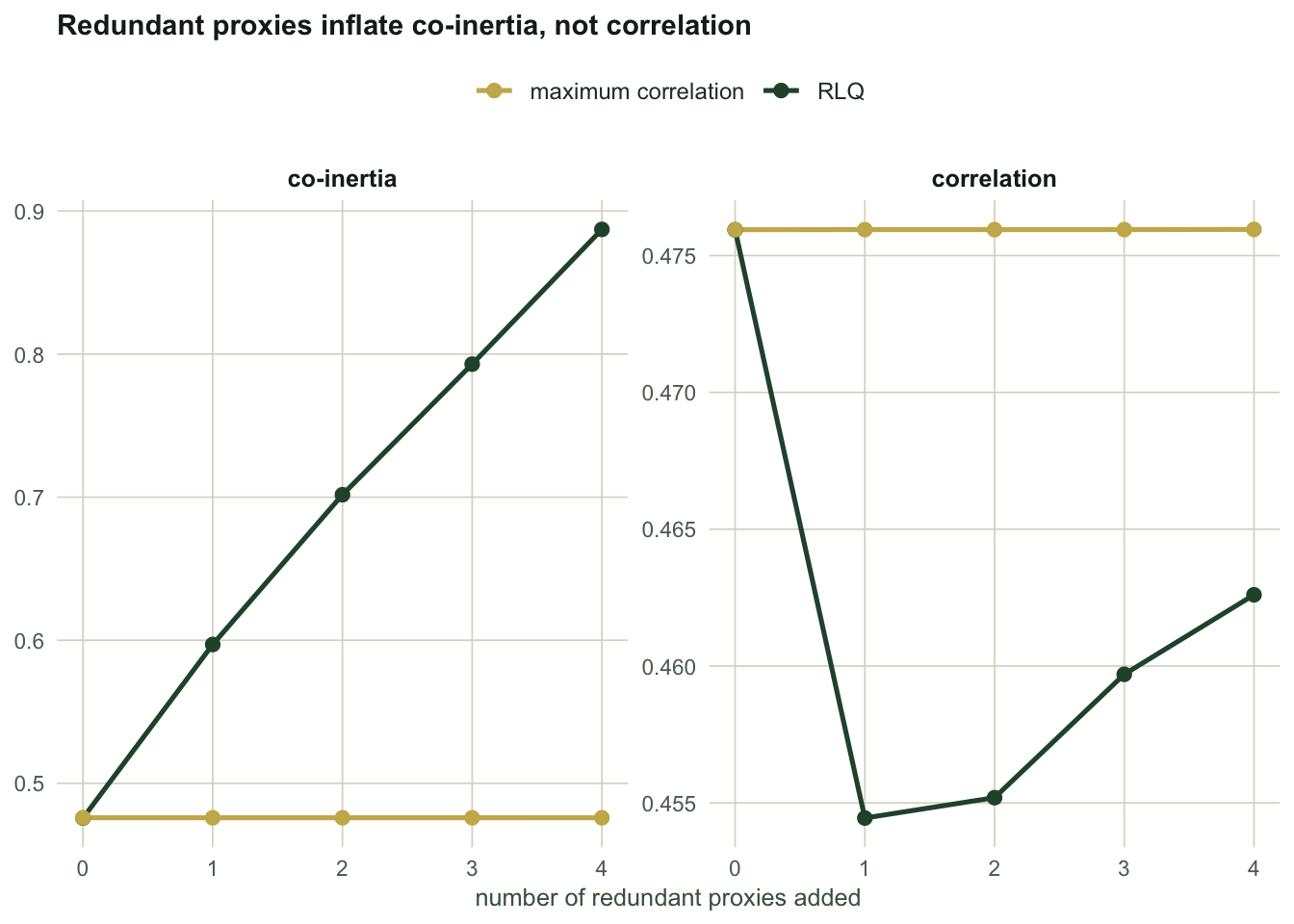
Read the columns. Every proxy is pure redundancy: correlated with elevation at 0.85, connected to no species, carrying no information the analysis did not already have. As they pile up:
- RLQ's co-inertia climbs from `r sprintf("%.3f", p311_c0)` to `r sprintf("%.3f", p311_c4)`, a rise of `r sprintf("%.0f%%", 100 * (p311_c4 / p311_c0 - 1))`.
- RLQ's correlation goes from `r sprintf("%.3f", p311_r0)` to `r sprintf("%.3f", p311_r4)`. It does not rise with the co-inertia; if anything it slips slightly, because the proxies dilute the axis.
- Elevation's loading on the axis, which has unit length, falls from `r sprintf("%.2f", p311_e0)` to `r sprintf("%.2f", p311_e4)`; squared, its share of the axis is `r sprintf("%.2f", p311_e4^2)`. The real driver is now a minority shareholder in the axis named after it.
- The correlation-maximising axis does not budge on any column.
```{r fig-sweep}
#| echo: false
#| fig-cap: "As redundant environmental proxies are added, RLQ's co-inertia climbs while its correlation stays flat. The correlation-maximising axis is invariant to both."
#| fig-alt: "Two line panels against number of proxies from zero to four. Left panel: RLQ co-inertia rises steadily from about 0.48 to 0.89 while the correlation-maximising co-inertia stays flat at about 0.48. Right panel: both correlations stay flat near 0.46 to 0.48 across all proxy counts."
library(ggplot2)
theme_te <- function() {
theme_minimal(base_size = 11) +
theme(
plot.background = element_rect(fill = "#f5f4ee", colour = NA),
panel.background = element_rect(fill = "#f5f4ee", colour = NA),
panel.grid.minor = element_blank(),
panel.grid.major = element_line(colour = "#dad9ca", linewidth = 0.3),
plot.title = element_text(colour = "#16241d", face = "bold", size = 11),
axis.title = element_text(colour = "#46604a", size = 9.5),
axis.text = element_text(colour = "#5d6b61", size = 8.5),
legend.position = "top", legend.title = element_blank(),
legend.text = element_text(colour = "#2c3a31", size = 9),
strip.text = element_text(colour = "#16241d", face = "bold", size = 9.5))
}
long <- rbind(
data.frame(proxies = sw$proxies, value = sw$rlq_coin, method = "RLQ", panel = "co-inertia"),
data.frame(proxies = sw$proxies, value = sw$cor_coin, method = "maximum correlation", panel = "co-inertia"),
data.frame(proxies = sw$proxies, value = sw$rlq_corr, method = "RLQ", panel = "correlation"),
data.frame(proxies = sw$proxies, value = sw$cor_corr, method = "maximum correlation", panel = "correlation"))
ggplot(long, aes(proxies, value, colour = method)) +
geom_line(linewidth = 0.9) + geom_point(size = 2.2) +
facet_wrap(~panel) +
scale_colour_manual(values = c("RLQ" = "#275139", "maximum correlation" = "#c9b458")) +
labs(title = "Redundant proxies inflate co-inertia, not correlation",
x = "number of redundant proxies added", y = NULL) +
theme_te()
```
## What this does not mean
RLQ is not broken, and this is not an argument against using it. Co-inertia is a defensible target: it asks how much trait-environment association there is *in total*, and a redundant proxy genuinely does add spread to the environmental table. If you report the co-inertia of a fitted RLQ as a measure of how much structure two tables share, the number is what it says it is.
What you cannot do is read the loadings as a statement about which environmental variable drives the community, or compare co-inertia values between analyses that used different numbers of correlated variables. Both readings are common and both are wrong for the same reason: the co-inertia depends on how you assembled the environmental table, not only on the ecology in it.
## Testing it
The permutation test for RLQ needs two nulls, not one, because the hypothesis is a conjunction: traits track the environment only if the environment relates to composition *and* the traits relate to composition. Shuffling sites tests the first link; shuffling species tests the second; the honest p-value is the larger of the two.
```{r perm}
rlq_stat <- function(R, L, Q) sum(rlq(R, L, Q)$d^2)
set.seed(311)
obs <- rlq_stat(R, L, Q)
nperm <- 199
ps <- replicate(nperm, rlq_stat(R[sample(n_site), ], L, Q))
pq <- replicate(nperm, rlq_stat(R, L, Q[sample(n_sp), ]))
p311_p_site <- (sum(ps >= obs) + 1) / (nperm + 1)
p311_p_sp   <- (sum(pq >= obs) + 1) / (nperm + 1)
p311_p_max  <- max(p311_p_site, p311_p_sp)
c(observed = obs, p_sites = p311_p_site, p_species = p311_p_sp, p_reported = p311_p_max)
```
Here both nulls reject, so the maximum rejects: `r sprintf("%.3f", p311_p_max)`. That is the easy case, where the link is real. The hard case is when only one of them rejects, and it is common enough that it has [its own post](../checking-a-trait-environment-analysis/), which measures how often each null alone gets it wrong. The short version: often. Report the maximum.
Note what the test does *not* fix. The permutation test asks whether the association is larger than chance. It says nothing about whether the axis you are about to interpret is loaded on the variable you think it is. Those are separate questions, and the sweep above is about the second one.
## Where to go next
If you want the axis to mean what you think it means, the correlation-maximising version is the one you want, and it is the subject of the [next post](../double-constrained-correspondence-analysis/). If you have one environmental variable and one trait, skip the ordination entirely and use [the fourth corner](../fourth-corner-trait-environment/): same covariance, no loadings to misread. If you want the plot-level trait average rather than an ordination axis, that is [the community weighted mean](../community-weighted-means/).
And if you keep only one thing: RLQ maximises covariance. Covariance is correlation times spread. Spread is something you control when you choose which columns go in the environmental table.
## References
Doledec S, Chessel D, ter Braak CJF, Champely S 1996 Environmental and Ecological Statistics 3:143-166 (10.1007/BF02427859)
Dray S, Chessel D, Thioulouse J 2003 Ecology 84:3078-3089 (10.1890/03-0178)
Dray S, Legendre P 2008 Ecology 89:3400-3412 (10.1890/08-0349.1)
Dray S, Choler P, Doledec S, Peres-Neto PR, Thuiller W, Pavoine S, ter Braak CJF 2014 Ecology 95:14-21 (10.1890/13-0196.1)
ter Braak CJF, Cormont A, Dray S 2012 Ecology 93(7):1525-1526 (10.1890/12-0126.1)
Dray S, Dufour AB 2007 Journal of Statistical Software 22:1-20 (10.18637/jss.v022.i04)
Legendre P, Legendre L 2012 Numerical Ecology, 3rd edition, ISBN 978-0-444-53868-0
## Related tutorials
- [The fourth corner statistic in R](../fourth-corner-trait-environment/)
- [Double constrained correspondence analysis in R](../double-constrained-correspondence-analysis/)
- [Community weighted means in R](../community-weighted-means/)
- [Checking a trait environment analysis](../checking-a-trait-environment-analysis/)