Double constrained correspondence analysis in R

dc-CA from scratch: whitening turns co-inertia into correlation, why that fixes RLQ’s proxy problem, and the symmetric trap it introduces instead.

RLQ maximises covariance, and covariance is correlation times spread. That has a consequence you can measure: adding a redundant environmental proxy inflates the co-inertia by adding spread, while the correlation stays where it was. The axis then loads on a variable that drives nothing.

Double constrained correspondence analysis fixes this by changing the objective. It maximises the correlation itself. This post builds it from scratch, shows the fix working, and then measures the price, which is real and symmetric: the same whitening that removes RLQ’s proxy problem manufactures correlation out of noise.

Where the name comes from

Ordinary CCA constrains one side: site scores are forced to be linear combinations of the environmental variables. Species scores stay free, so they absorb whatever they like. dc-CA constrains both sides. Site scores must be built from the environment; species scores must be built from the traits. That is the double constraint, and it is why the method belongs in the trait-environment family rather than the ordination family.

The consequence is that the axis has a specific meaning. The site score is an environmental gradient. The species score is a trait axis. The eigenvalue is the correlation between them, computed through the community table. That is the fourth corner correlation, for the best pair of composite variables the two tables can build.

Setup

Same data-generating process as the RLQ post: sixty sites on an elevation gradient, forty species whose optima are set by their SLA.

set.seed(3120)
n_site <- 60; n_sp <- 40

elev_z <- as.numeric(scale(seq(-2, 2, length.out = n_site) + rnorm(n_site, 0, 0.25)))
sla_z  <- as.numeric(scale(rnorm(n_sp)))
seed_z <- as.numeric(scale(rnorm(n_sp)))
opt <- -1.2 * sla_z + rnorm(n_sp, 0, 0.4)

L <- matrix(0, n_site, n_sp)
for (j in 1:n_sp) L[, j] <- rpois(n_site, 25 * exp(-(elev_z - opt[j])^2 / (2 * 0.9^2)))
keep <- colSums(L) > 0
L <- L[, keep]; sla_z <- sla_z[keep]; seed_z <- seed_z[keep]
n_sp <- ncol(L)
Q <- cbind(SLA = sla_z, seed_mass = seed_z)
c(sites = n_site, species = n_sp)

  sites species 
     60      40 

The machine

Everything up to the cross table is identical to RLQ. One extra step turns it into dc-CA.

ca_weights <- function(L) {
  P <- L / sum(L)
  r <- rowSums(P); cw <- colSums(P)
  list(r = r, c = cw, Z = P / outer(r, cw) - 1, P = P)
}
wstd <- function(X, w) {
  Xc <- sweep(X, 2, colSums(X * w))
  sweep(Xc, 2, sqrt(colSums(Xc^2 * w)), "/")
}
msqrt_inv <- function(M) {          # inverse matrix square root
  e <- eigen(M, symmetric = TRUE)
  d <- 1 / sqrt(pmax(e$values, 1e-10))
  # d * t(e$vectors) is diag(d) %*% t(e$vectors) without building diag(d):
  # diag() of a length-1 vector returns an identity matrix, not a 1x1 matrix
  e$vectors %*% (d * t(e$vectors))
}

dcca <- function(R, L, Q) {
  ca <- ca_weights(L)
  Rw <- wstd(R, ca$r); Qw <- wstd(Q, ca$c)
  Zm <- t(Rw * ca$r) %*% ca$Z %*% (Qw * ca$c)      # the same cross table as RLQ
  CR <- t(Rw * ca$r) %*% Rw                        # weighted covariance of R
  CQ <- t(Qw * ca$c) %*% Qw                        # weighted covariance of Q
  Ar <- msqrt_inv(CR); Aq <- msqrt_inv(CQ)
  s <- svd(Ar %*% Zm %*% Aq)                       # THE step: whiten, then decompose
  list(d = s$d, u = Ar %*% s$u, v = Aq %*% s$v, ca = ca, Rw = Rw, Qw = Qw, Z = Zm)
}

That single line is the whole difference. RLQ decomposes the cross table as it stands, so directions with more spread win. dc-CA divides the spread out of both sides first, so only the correlation is left to maximise. The singular values of the whitened cross table are correlations, bounded by one, and you can check that directly:

fitR <- cbind(elevation = elev_z, slope = as.numeric(scale(rnorm(n_site))))
f <- dcca(fitR, L, Q)
sR <- as.numeric(f$Rw %*% f$u[, 1]); sQ <- as.numeric(f$Qw %*% f$v[, 1])
vR <- sum(sR^2 * f$ca$r); vQ <- sum(sQ^2 * f$ca$c)
cv <- sum((sR %o% sQ) * f$ca$P) - sum(sR * f$ca$r) * sum(sQ * f$ca$c)
p312_corr <- cv / sqrt(vR * vQ)
p312_d1 <- f$d[1]
p312_gap <- abs(p312_corr - p312_d1)
c(eigenvalue = p312_d1, correlation_of_scores = p312_corr, gap = p312_gap)

           eigenvalue correlation_of_scores                   gap 
         5.922591e-01          5.922591e-01          4.440892e-16 

The first eigenvalue is 0.5923 and the correlation between the two sets of scores is 0.5923. The gap is 4.4e-16. The eigenvalue is not related to the correlation; it is the correlation.

The fix, working

Rerun the RLQ proxy sweep on dc-CA. Each proxy correlates with elevation at 0.85 and affects nothing.

sweep_proxy <- function(nproxy, rho = 0.85) {
  set.seed(77)
  Rm <- cbind(elevation = elev_z)
  for (k in seq_len(nproxy))
    Rm <- cbind(Rm, as.numeric(scale(rho * elev_z + rnorm(n_site, 0, sqrt(1 - rho^2)))))
  pn <- if (nproxy > 0) paste0("proxy", seq_len(nproxy)) else character(0)
  colnames(Rm) <- c("elevation", pn)
  f <- dcca(Rm, L, Q)
  ld <- f$u[, 1] / sqrt(sum(f$u[, 1]^2))
  data.frame(proxies = nproxy, dcca_corr = f$d[1], elevation_share = abs(ld[1]))
}
sp <- do.call(rbind, lapply(0:4, sweep_proxy))
p312_sp <- sp
print(round(sp, 4), row.names = FALSE)

 proxies dcca_corr elevation_share
       0    0.5919          1.0000
       1    0.5919          1.0000
       2    0.5920          0.9999
       3    0.5920          0.9996
       4    0.5920          0.9996

The correlation is flat and elevation keeps essentially the whole axis. Whitening removed the incentive to recruit redundant variables, because a redundant variable adds spread and dc-CA does not reward spread. This is the honest advantage of dc-CA over RLQ, and it is the reason ter Braak and colleagues argue for it.

Now the other half of the ledger.

The price: correlation from nothing

Whitening buys degrees of freedom. When you invert the covariance matrix of the environmental table, you are letting the method search a larger space for a direction that lines up with the traits, and a large enough space always contains one. Watch what happens with an environmental table made entirely of noise, unconnected to anything.

sweep_noise <- function(p) {
  set.seed(900 + p)
  Rn <- matrix(rnorm(n_site * p), n_site)
  colnames(Rn) <- paste0("noise", seq_len(p))
  Rreal <- cbind(elevation = elev_z, Rn[, -1, drop = FALSE])
  data.frame(n_env_vars = p,
             with_real_driver = dcca(Rreal, L, Q)$d[1],
             noise_only = dcca(Rn, L, Q)$d[1])
}
ns <- do.call(rbind, lapply(c(1, 3, 6, 12, 20), sweep_noise))
p312_ns <- ns
p312_n1 <- ns$noise_only[1]; p312_n20 <- ns$noise_only[5]
p312_real <- ns$with_real_driver[5]
print(round(ns, 4), row.names = FALSE)

 n_env_vars with_real_driver noise_only
          1           0.5919     0.0104
          3           0.5919     0.0398
          6           0.5920     0.1385
         12           0.5926     0.2709
         20           0.5926     0.3399

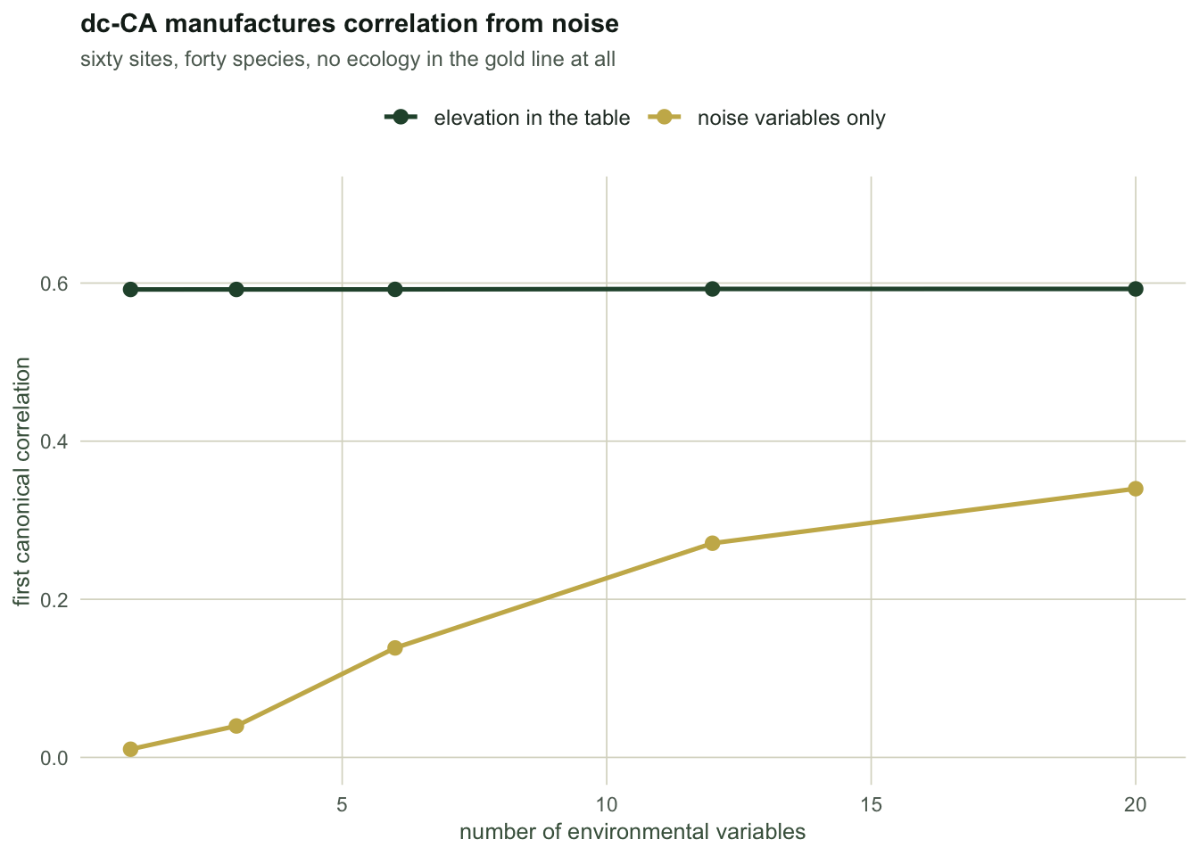
With one noise variable the first canonical correlation is 0.010, which is honest: there is nothing there. With twenty, it is 0.340. Nothing changed in the ecology. The community still responds to elevation, elevation is still absent from the table, and the twenty columns are still independent standard normals. dc-CA manufactured a moderate trait-environment correlation out of the arithmetic.

Note also the middle column: the real signal sits at about 0.593 and does not care how many noise columns ride along. Noise variables do not corrupt a real signal. They fabricate one when there is none, which is worse, because that is exactly the case where you have no prior to check the number against.

Figure 1: First canonical correlation from dc-CA as noise environmental variables are added. The real signal is stable; the noise-only line climbs from nothing.

This is the exact mirror of RLQ’s problem. RLQ inflates with redundant variables because it rewards spread. dc-CA inflates with any variables because it rewards fit. Neither method is broken; each one has an objective, and each objective has a way of being gamed by the shape of the table you feed it.

The test that saves both

The permutation test is not decoration here. It is the thing that separates 0.340 from a finding.

Two nulls, because the hypothesis is a conjunction. Shuffling sites breaks the environment-composition link while keeping the trait-composition link. Shuffling species does the reverse. The reported p-value is the larger of the two, which is ter Braak, Cormont and Dray’s model 6.

dcca_d1 <- function(R, L, Q) dcca(R, L, Q)$d[1]
perm_test <- function(R, L, Q, nperm = 199, seed = 1) {
  set.seed(seed)
  obs <- dcca_d1(R, L, Q)
  ps <- replicate(nperm, dcca_d1(R[sample(nrow(R)), , drop = FALSE], L, Q))
  pq <- replicate(nperm, dcca_d1(R, L, Q[sample(nrow(Q)), , drop = FALSE]))
  c(observed = obs,
    p_sites = (sum(ps >= obs) + 1) / (nperm + 1),
    p_species = (sum(pq >= obs) + 1) / (nperm + 1))
}
set.seed(920)
Rnoise <- matrix(rnorm(n_site * 20), n_site); colnames(Rnoise) <- paste0("noise", 1:20)
a <- perm_test(Rnoise, L, Q, seed = 1)
b <- perm_test(cbind(elevation = elev_z, Rnoise[, 1:2]), L, Q, seed = 2)
p312_a <- a; p312_b <- b
p312_a_max <- max(a["p_sites"], a["p_species"])
p312_b_max <- max(b["p_sites"], b["p_species"])
rbind(`noise only, 20 vars` = c(a, reported = p312_a_max),
      `elevation + 2 noise` = c(b, reported = p312_b_max))

                     observed p_sites p_species reported
noise only, 20 vars 0.3399189   0.395     0.005    0.395
elevation + 2 noise 0.5919434   0.005     0.005    0.005

Read the noise-only row carefully, because it is the whole argument for the two-null rule.

The observed correlation is 0.340. The site-shuffle null gives p = 0.395: it says, correctly, that this is what twenty noise columns produce. The species-shuffle null gives p = 0.005, which is a false positive at any threshold anyone uses. Had you run one permutation test, the standard one, you would have had a publishable trait-environment result from a table of random numbers.

The maximum reports 0.395, and the analysis stops where it should.

Why the species null misfires

It is worth seeing the mechanism rather than trusting the rule, because the same mechanism will bite you in other places.

set.seed(3)
nperm <- 199
obs_n <- dcca_d1(Rnoise, L, Q)
ns_site <- replicate(nperm, dcca_d1(Rnoise[sample(n_site), ], L, Q))
ns_sp   <- replicate(nperm, dcca_d1(Rnoise, L, Q[sample(n_sp), ]))
p312_null <- data.frame(
  null = c("shuffle sites", "shuffle species"),
  mean = c(mean(ns_site), mean(ns_sp)),
  sd = c(sd(ns_site), sd(ns_sp)),
  q95 = c(quantile(ns_site, 0.95), quantile(ns_sp, 0.95)))
p312_obs_n <- obs_n
print(round(p312_null[, -1], 4), row.names = FALSE)

  mean     sd    q95
 0.335 0.0429 0.4040
 0.088 0.0340 0.1472

The observed value is 0.3399. The site-shuffle null is centred at 0.3350, so the observed value sits in the middle of it. That null preserves the whitening inflation, because shuffling the rows of a noise table produces another noise table.

The species-shuffle null is centred at 0.0880, a factor of 3.8 lower. Shuffling species destroys the trait gradient, and the trait gradient was doing the work. With real traits, the community-weighted trait score varies smoothly across sites, and a smooth sixty-point curve is easy for twenty noise columns to chase. Scramble the traits and that curve becomes a jagged one, which twenty noise columns fit far less well.

So the species null is not measuring the reference distribution of the statistic. It is measuring a different, easier problem, and it declares the observed value extreme because the observed value came from the harder one. That is the same failure the fourth corner shows, on a different statistic, and it is measured in detail elsewhere.

Which one should you use

Both, and mostly for different questions.

Use dc-CA when the axis needs to mean something: when you will write a sentence naming an environmental variable and a trait, and expect the reader to believe the pairing. Its axis loads on what actually predicts, not on what happens to be correlated with what predicts.

Use RLQ when you want to describe the total shared structure between two tables and are willing to read the co-inertia as a summary rather than an attribution. Its output is also more forgiving with small samples, since it does not invert anything.

And in either case, the number that decides whether there is anything to interpret is the permutation p-value, taken as the maximum of two nulls, not the eigenvalue.

The honest limit

Neither method identifies a mechanism. The best case is that you have measured an association between a trait axis and an environmental axis, weighted by abundance. The association could be driven by a variable you did not measure, by shared phylogeny among the species carrying the trait, or by the trait being a proxy for the thing that actually matters. Ordination cannot tell you which, and no permutation test can either: shuffling changes the null, not the causal structure.

There is also a sample size floor that neither the eigenvalue nor the p-value advertises. dc-CA inverts a covariance matrix, and with many environmental variables relative to sites, that inversion becomes unstable long before it becomes impossible. The noise sweep above is that instability, measured. If your environmental table has twenty columns and sixty sites, the honest move is to cut the table on ecological grounds before you fit, not to fit and then admire the eigenvalue.

References

ter Braak, Smilauer & Dray 2018 Environmental and Ecological Statistics 25(2):171-197 (10.1007/s10651-017-0395-x)

ter Braak, Peres-Neto & Dray 2018 Journal of Vegetation Science 29(5):801-811 (10.1111/jvs.12666)

ter Braak, Cormont & Dray 2012 Ecology 93(7):1525-1526 (10.1890/12-0126.1)

Dray & Legendre 2008 Ecology 89:3400-3412 (10.1890/08-0349.1)

Dray, Choler, Doledec, Peres-Neto, Thuiller, Pavoine & ter Braak 2014 Ecology 95:14-21 (10.1890/13-0196.1)

Doledec, Chessel, ter Braak & Champely 1996 Environmental and Ecological Statistics 3:143-166 (10.1007/BF02427859)

Peres-Neto, Dray & ter Braak 2017 Ecography 40(7):806-816 (10.1111/ecog.02302)

Related tutorials

• RLQ analysis in R: traits, sites and environment
• The fourth corner statistic in R
• Checking a trait environment analysis
• RDA, CCA and gradient length