library(ggplot2)

te_pal <- list(forest = "#275139", green = "#2f8f63", sage = "#93a87f",
               clay = "#b5534e", gold = "#cda23f", line = "#dad9ca",
               ink = "#16241d", paper = "#f5f4ee")

theme_te <- function() {
  theme_minimal(base_size = 12) +
    theme(panel.grid.minor = element_blank(),
          panel.grid.major = element_line(colour = "#e7e6dc"),
          plot.background = element_rect(fill = "#f5f4ee", colour = NA),
          panel.background = element_rect(fill = "#f5f4ee", colour = NA),
          plot.title = element_text(face = "bold", colour = te_pal$ink),
          axis.title = element_text(colour = te_pal$ink),
          legend.position = "bottom")
}Range size distributions
R
macroecology
biogeography
ecology tutorial
ggplot2
Measure geographic range sizes in a simulated atlas and see how grid grain, recording effort and the choice between AOO and EOO reshape the small-range tail.
The atlas arrives as a spreadsheet with three columns: species, grid cell, date. Somebody has spent thirty years filling it in. The regional red list has to come out of it, and the first thing anyone does with an atlas is count cells per species and sort the result. Most species turn out to occupy a handful of cells. A few occupy nearly everything. The histogram of those counts, on a log axis, is the range size distribution, and it has the same shape in almost every atlas anyone has compiled: hard right skew on the raw scale, close to symmetric once you take logs.
That shape is not a curiosity. The left end of it is the list of species that will be assessed against the IUCN thresholds, and two of those thresholds are areas: 2000 square kilometres of area of occupancy for Vulnerable, 500 for Endangered. A species falls on one side of a line or the other, and the number that decides it comes out of the same spreadsheet.
The claim this post makes is that the number is not a measurement. A geographic range size is constructed, and three of the construction decisions move the small-range end of the distribution further than anything biological in the data does. The first is grain: how big the grid cell is. The second is effort: how many records the species has. The third is which quantity you compute, because area of occupancy and extent of occurrence are different areas and they disagree most for exactly the species that matter.
Each of those is measured here rather than asserted. The atlas is simulated, for the reason it always is: a simulated atlas has a truth column, so an estimated range can be divided by the range the species actually has, and the answer is a number rather than an opinion. Nothing in the generator is adversarial. The species have smooth environmental preferences, limited geographic extents, patchy occupancy inside those extents and a few outlying populations, which is what atlas distributions look like.
The species-area curve is a different relationship built from the same kind of grid data and it has its own post, species-area relationships; this one is about the distribution of range sizes across species rather than the accumulation of species with area. If what you want is the abundance side of the same coin, the abundance-occupancy relationship is the neighbouring post, and it matters here because it is the reason recording effort is not spread evenly across the small-range tail.
An atlas with a truth column
The region is a square grid of 2 km cells, the resolution the IUCN guidelines recommend for area of occupancy, and it is 128 cells on a side. Two smooth environmental surfaces run across it, built as sums of low frequency waves so that neighbouring cells resemble each other. Every species gets an environmental optimum, a tolerance around it, a geographic centre and a geographic extent; the probability that it occupies a cell is the product of an environmental term, a distance term and a per species occupancy constant. A minority of species also get one to three outlying populations, placed two to four extents away from the centre, because real ranges have those and they are what makes the two area measures diverge.
set.seed(20260725)

nx <- 128
ny <- 128
cell_km <- 2
cell_area <- cell_km^2
gx <- rep(seq_len(nx), ny)
gy <- rep(seq_len(ny), each = nx)
n_cell <- nx * ny
region_area <- n_cell * cell_area
n_sp <- 200

# whole numbers quoted in the prose are written out in full rather than in R's
# scientific shorthand, so that 65536 does not turn up as 6.5536e4
n0 <- function(x) format(round(unname(x)), scientific = FALSE, trim = TRUE)

smooth_field <- function(nk = 5) {
  f <- numeric(n_cell)
  for (k in seq_len(nk)) {
    u <- sample(1:3, 1)
    v <- sample(1:3, 1)
    ph <- runif(2, 0, 2 * pi)
    a <- rnorm(1)
    f <- f + a * cos(2 * pi * u * gx / nx + ph[1]) *
      cos(2 * pi * v * gy / ny + ph[2])
  }
  as.numeric(scale(f))
}
E1 <- smooth_field()
E2 <- smooth_field()

ctr <- sample(n_cell, n_sp, replace = TRUE)
m1 <- E1[ctr] + rnorm(n_sp, 0, 0.2)
m2 <- E2[ctr] + rnorm(n_sp, 0, 0.2)
tol <- exp(rnorm(n_sp, log(0.85), 0.55))
rad <- exp(rnorm(n_sp, log(11), 1.0))
hold <- runif(n_sp, 0.25, 0.95)
n_out <- rbinom(n_sp, 3, 0.16)

occ <- vector("list", n_sp)
for (i in seq_len(n_sp)) {
  dg <- sqrt((gx - gx[ctr[i]])^2 + (gy - gy[ctr[i]])^2)
  de <- sqrt((E1 - m1[i])^2 + (E2 - m2[i])^2)
  p <- hold[i] * exp(-de^2 / (2 * tol[i]^2)) * exp(-dg^2 / (2 * rad[i]^2))
  keep <- which(runif(n_cell) < p)
  if (!length(keep)) keep <- ctr[i]
  if (n_out[i] > 0) {
    ang <- runif(n_out[i], 0, 2 * pi)
    rr <- rad[i] * runif(n_out[i], 2, 4)
    ox <- pmin(nx, pmax(1, round(gx[ctr[i]] + rr * cos(ang))))
    oy <- pmin(ny, pmax(1, round(gy[ctr[i]] + rr * sin(ang))))
    keep <- unique(c(keep, (oy - 1) * nx + ox))
  }
  occ[[i]] <- keep
}
nocc <- lengths(occ)
aoo <- nocc * cell_area

round(c(species = n_sp, grid_cells = n_cell, cell_side_km = cell_km,
        cell_area_km2 = cell_area, region_area_km2 = region_area,
        smallest_aoo_km2 = min(aoo), median_aoo_km2 = median(aoo),
        largest_aoo_km2 = max(aoo),
        species_in_a_single_cell = sum(nocc == 1),
        widest_species_share_of_region = max(aoo) / region_area,
        mean_of_log_aoo = mean(log(aoo)), sd_of_log_aoo = sd(log(aoo))), 4)
species grid_cells
200.0000 16384.0000
cell_side_km cell_area_km2
2.0000 4.0000
region_area_km2 smallest_aoo_km2
65536.0000 4.0000
median_aoo_km2 largest_aoo_km2
442.0000 18996.0000
species_in_a_single_cell widest_species_share_of_region
2.0000 0.2899
mean_of_log_aoo sd_of_log_aoo
6.0367 1.5828 print(round(quantile(aoo, c(0.05, 0.25, 0.5, 0.75, 0.95)), 1)) 5% 25% 50% 75% 95%
35.8 148.0 442.0 1157.0 5419.4 Two hundred species on a region of 65536 square kilometres. The smallest occupies a single cell, 4 square kilometres, and the largest occupies 18996 square kilometres, which is 29.0 per cent of the region. The median species sits at 442. That is the atlas, and everything after this is derived from it.
Two measures on one map
Area of occupancy is the easy one: count the occupied cells and multiply by the cell area. Extent of occurrence is the area of the convex hull of the occurrences, the smallest convex polygon containing them all. Base R has both halves. chull returns the indices of the points on the hull, in order round it, and the shoelace formula turns an ordered polygon into an area.
The shoelace formula is worth writing out rather than importing, because it is three lines and because a routine that returns an area should be calibrated before it is trusted. A square of side 10 has an area of 100 and a triangle with legs 30 and 20 has an area of 300; both are printed beside what the function returns. The third check adds a point in the middle of the square: chull has to ignore it, because it is not a vertex of anything.
poly_area <- function(x, y) {
  n <- length(x)
  if (n < 3) return(NA_real_)
  j <- c(n, seq_len(n - 1))
  abs(sum(x[j] * y - x * y[j])) / 2
}

hull_area <- function(x, y) {
  if (length(x) < 3) return(NA_real_)
  h <- chull(x, y)
  if (length(h) < 3) return(NA_real_)
  poly_area(x[h], y[h])
}

sq_x <- c(0, 10, 10, 0)
sq_y <- c(0, 0, 10, 10)
tri_x <- c(0, 30, 0)
tri_y <- c(0, 0, 20)

round(c(square_from_the_shoelace = poly_area(sq_x, sq_y),
        square_exact = 10 * 10,
        square_with_the_vertices_reversed = poly_area(rev(sq_x), rev(sq_y)),
        triangle_from_the_shoelace = poly_area(tri_x, tri_y),
        triangle_exact = 30 * 20 / 2,
        square_plus_an_interior_point = hull_area(c(sq_x, 5), c(sq_y, 5)),
        two_points_only = hull_area(c(0, 1), c(0, 1))), 4)
square_from_the_shoelace square_exact
100 100
square_with_the_vertices_reversed triangle_from_the_shoelace
100 300
triangle_exact square_plus_an_interior_point
300 100
two_points_only
NA eoo <- vapply(occ, function(k) hull_area(gx[k] * cell_km, gy[k] * cell_km), 1)
packing <- aoo / eoo
n_no_hull <- sum(is.na(eoo))
round(c(species_with_a_defined_eoo = sum(!is.na(eoo)),
species_with_fewer_than_three_cells = n_no_hull,
median_eoo_km2 = median(eoo, na.rm = TRUE),
smallest_eoo_km2 = min(eoo, na.rm = TRUE),
largest_eoo_km2 = max(eoo, na.rm = TRUE),
median_eoo_over_aoo = median(eoo / aoo, na.rm = TRUE),
smallest_eoo_over_aoo = min(eoo / aoo, na.rm = TRUE),
largest_eoo_over_aoo = max(eoo / aoo, na.rm = TRUE)), 4) species_with_a_defined_eoo species_with_fewer_than_three_cells
197.0000 3.0000
median_eoo_km2 smallest_eoo_km2
3784.0000 2.0000
largest_eoo_km2 median_eoo_over_aoo
64494.0000 7.6151
smallest_eoo_over_aoo largest_eoo_over_aoo
0.1667 102.4868 The calibration passes: 100 against 100, 300 against 300, and reversing the vertex order changes nothing because the absolute value takes care of the sign. The hull of the square with a point added at its centre is still 100. Two points return NA rather than zero, which is the honest answer, because a convex hull needs three points that are not collinear and 3 species in this atlas do not have them.
Across the atlas the median extent of occurrence is 3784 square kilometres against a median area of occupancy of 442. Two species with almost the same area of occupancy can have extents that differ by a large factor. The map picks the pair out: among species occupying between 100 and 400 cells, the one whose occupied cells pack most tightly inside their own hull, and the one whose pack most loosely.
cand <- which(nocc >= 100 & nocc <= 400 & !is.na(eoo))
sp_tight <- cand[which.max(packing[cand])]
sp_loose <- cand[which.min(packing[cand])]
pair_aoo_ratio <- aoo[sp_loose] / aoo[sp_tight]
pair_eoo_ratio <- eoo[sp_loose] / eoo[sp_tight]

round(c(tight_species = sp_tight, tight_cells = nocc[sp_tight],
        tight_aoo_km2 = aoo[sp_tight], tight_eoo_km2 = eoo[sp_tight],
        tight_eoo_over_aoo = eoo[sp_tight] / aoo[sp_tight],
        loose_species = sp_loose, loose_cells = nocc[sp_loose],
        loose_aoo_km2 = aoo[sp_loose], loose_eoo_km2 = eoo[sp_loose],
        loose_eoo_over_aoo = eoo[sp_loose] / aoo[sp_loose],
        ratio_of_the_two_aoo = pair_aoo_ratio,
        ratio_of_the_two_eoo = pair_eoo_ratio), 4)
tight_species tight_cells tight_aoo_km2
65.0000 127.0000 508.0000
tight_eoo_km2 tight_eoo_over_aoo loose_species
1314.0000 2.5866 170.0000
loose_cells loose_aoo_km2 loose_eoo_km2
150.0000 600.0000 36284.0000
loose_eoo_over_aoo ratio_of_the_two_aoo ratio_of_the_two_eoo
60.4733 1.1811 27.6134 map_one <- function(i, lab) {
k <- occ[[i]]
h <- chull(gx[k], gy[k])
rbind(data.frame(x = gx[k] * cell_km, y = gy[k] * cell_km, part = "cell",
panel = lab),
data.frame(x = gx[k][h] * cell_km, y = gy[k][h] * cell_km,
part = "hull", panel = lab))
}
lab_tight <- "Tightly packed species"
lab_loose <- "Loosely packed species"
md <- rbind(map_one(sp_tight, lab_tight), map_one(sp_loose, lab_loose))
md$panel <- factor(md$panel, levels = c(lab_tight, lab_loose))
# the occupied patch is small against a 256 km square, so each panel states its
# own cell count and hull area rather than leaving them to be judged by eye
say <- function(i) sprintf("%s cells, %s km2 occupied\nhull %s km2",
n0(nocc[i]), n0(aoo[i]), n0(eoo[i]))
map_lab <- data.frame(x = 248, y = 6, panel = factor(c(lab_tight, lab_loose),
levels = c(lab_tight, lab_loose)),
txt = c(say(sp_tight), say(sp_loose)))
ggplot() +
geom_tile(data = md[md$part == "cell", ],
aes(x, y, fill = "Occupied 2 km cell"),
width = cell_km, height = cell_km, colour = te_pal$forest,
linewidth = 0.35) +
geom_polygon(data = md[md$part == "hull", ],
aes(x, y, colour = "Convex hull (extent of occurrence)"),
fill = NA, linewidth = 0.7) +
geom_text(data = map_lab, aes(x, y, label = txt), hjust = 1, vjust = 0,
size = 2.9, lineheight = 0.95, colour = te_pal$ink) +
facet_wrap(~panel) +
coord_fixed(xlim = c(0, nx * cell_km), ylim = c(0, ny * cell_km)) +
scale_fill_manual(values = te_pal$forest, name = NULL) +
scale_colour_manual(values = te_pal$clay, name = NULL) +
scale_x_continuous(breaks = seq(0, 256, 64)) +
scale_y_continuous(breaks = seq(0, 256, 64)) +
labs(x = "Easting (km)", y = "Northing (km)",
title = "Same area of occupancy, very different extent") +
theme_te() +
theme(strip.text = element_text(colour = te_pal$ink, face = "bold",
size = 9),
legend.box = "vertical",
legend.margin = margin(0, 0, 0, 0),
plot.margin = margin(6, 12, 6, 6))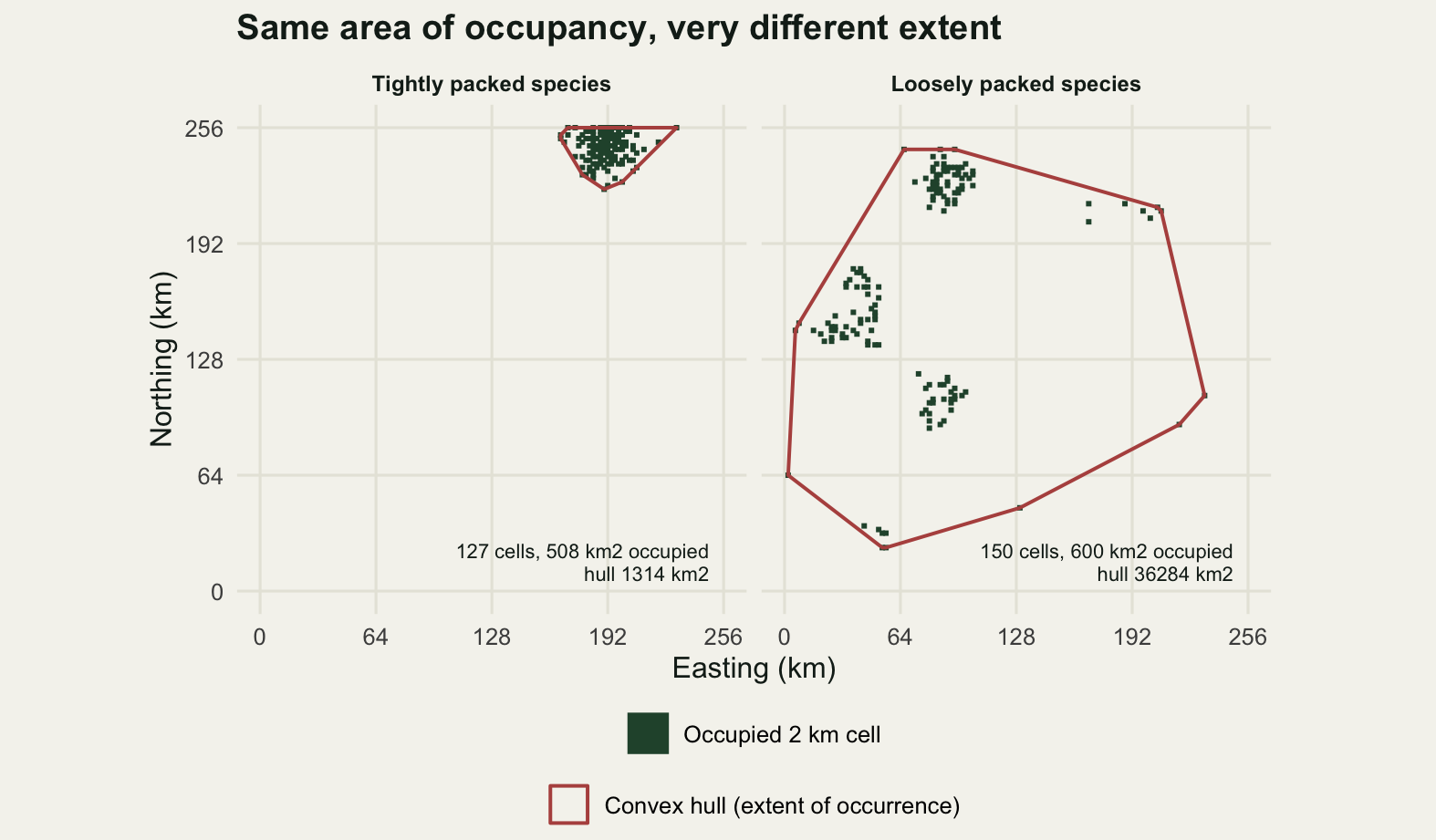
Species 65 occupies 127 cells and species 170 occupies 150, so their areas of occupancy differ by a factor of 1.1811. Their extents of occurrence differ by a factor of 27.6134. The loose one is not a wider ranging species in any sense the cells support; it is the same amount of occupied ground with more distance between the pieces.
The shape of the distribution and what it is evidence for
Take logs and plot the histogram. It is close to symmetric, which is the observation reported from atlas after atlas since the 1990s and usually written up as the range size distribution being lognormal. The maximum likelihood fit of a lognormal is two lines of arithmetic: the mean and the uncorrected standard deviation of the logged values are the estimates.
The question is what that fit is evidence for. A right-skewed positive quantity is what any product of several independent positive factors produces, and a geographic range is a product of several: climatic tolerance times dispersal ability times habitat availability times how long the species has been in the region. So the test that matters is not whether a lognormal fits, but whether the data can tell a lognormal from anything else. Two comparisons are run. The first fits a log-logistic in place of the lognormal, which is the same idea with a slightly heavier pair of tails, and prints the difference in AIC. The second generates range sizes from a genuinely different process, a product of six independent uniform factors rescaled to the same mean and spread on the log scale, and fits both families to that as well.
set.seed(4404)

y <- log(aoo)
mu <- mean(y)
sigma <- sqrt(mean((y - mu)^2))
ll_lnorm <- sum(dlnorm(aoo, mu, sigma, log = TRUE))

fit_loglogis <- function(a) {
  yy <- log(a)
  optim(c(mean(yy), log(sd(yy) * sqrt(3) / pi)),
        function(p) -sum(dlogis(yy, p[1], exp(p[2]), log = TRUE) - yy),
        method = "Nelder-Mead")
}
f_ll <- fit_loglogis(aoo)
loc <- f_ll$par[1]
scl <- exp(f_ll$par[2])
ll_llogis <- -f_ll$value
d_atlas <- 2 * (ll_lnorm - ll_llogis)

prod6 <- apply(matrix(runif(n_sp * 6, 0.15, 2.2), ncol = 6), 1, prod)
alt <- exp(mu + sigma * (log(prod6) - mean(log(prod6))) / sd(log(prod6)))
ya <- log(alt)
mu_a <- mean(ya)
sig_a <- sqrt(mean((ya - mu_a)^2))
d_alt <- 2 * (sum(dlnorm(alt, mu_a, sig_a, log = TRUE)) +
                fit_loglogis(alt)$value)

nq <- qnorm(ppoints(n_sp))
qq_atlas <- cor(sort(y), nq)
qq_alt <- cor(sort(ya), nq)

round(c(lognormal_mu = mu, lognormal_sigma = sigma,
        lognormal_loglik = ll_lnorm,
        loglogistic_location = loc, loglogistic_scale = scl,
        loglogistic_loglik = ll_llogis,
        parameters_in_each = 2,
        delta_aic_atlas = d_atlas,
        delta_aic_multiplicative_sample = d_alt,
        normal_qq_correlation_atlas = qq_atlas,
        normal_qq_correlation_multiplicative = qq_alt,
        skew_of_log_aoo = mean((y - mu)^3) / sd(y)^3,
        skew_of_the_multiplicative_sample = mean((ya - mu_a)^3) / sd(ya)^3,
        optimiser_converged = f_ll$convergence), 4)
lognormal_mu lognormal_sigma
6.0367 1.5789
lognormal_loglik loglogistic_location
-1582.4640 6.0513
loglogistic_scale loglogistic_loglik
0.8935 -1583.2692
parameters_in_each delta_aic_atlas
2.0000 1.6104
delta_aic_multiplicative_sample normal_qq_correlation_atlas
5.8681 0.9973
normal_qq_correlation_multiplicative skew_of_log_aoo
0.9952 -0.1396
skew_of_the_multiplicative_sample optimiser_converged
-0.2836 0.0000 set.seed(1808)
pick <- function(a) {
yy <- log(a)
m <- mean(yy)
s <- sqrt(mean((yy - m)^2))
c(sum(dlnorm(a, m, s, log = TRUE)), -fit_loglogis(a)$value)
}
n_rep <- 400
right <- matrix(NA, n_rep, 2)
gap <- numeric(n_rep)
for (r in seq_len(n_rep)) {
v1 <- pick(rlnorm(n_sp, mu, sigma))
v2 <- pick(exp(rlogis(n_sp, loc, scl)))
right[r, 1] <- v1[1] > v1[2]
right[r, 2] <- v2[2] > v2[1]
gap[r] <- 2 * (v1[1] - v1[2])
}
pc_lnorm <- 100 * mean(right[, 1])
pc_llogis <- 100 * mean(right[, 2])
pc_both <- 100 * mean(right)
med_gap <- median(gap)
round(c(replicates = n_rep, species_per_replicate = n_sp,
percent_correct_when_lognormal_is_true = pc_lnorm,
percent_correct_when_loglogistic_is_true = pc_llogis,
percent_correct_overall = pc_both,
median_delta_aic_when_lognormal_is_true = med_gap,
lower_quartile_of_that_delta = quantile(gap, 0.25),
observed_delta_aic_in_the_atlas = d_atlas), 4) replicates
400.0000
species_per_replicate
200.0000
percent_correct_when_lognormal_is_true
87.5000
percent_correct_when_loglogistic_is_true
80.7500
percent_correct_overall
84.1250
median_delta_aic_when_lognormal_is_true
4.3150
lower_quartile_of_that_delta.25%
2.2029
observed_delta_aic_in_the_atlas
1.6104 xs <- seq(min(log10(c(aoo, alt))) - 0.3, max(log10(c(aoo, alt))) + 0.3,
length.out = 400)
keys <- c("Lognormal fit", "Log-logistic fit", "Multiplicative sample")
curve_df <- data.frame(
x = rep(xs, 2),
d = c(log(10) * dnorm(xs * log(10), mu, sigma),
log(10) * dlogis(xs * log(10), loc, scl)),
fit = factor(rep(keys[1:2], each = length(xs)), levels = keys))
alt_df <- data.frame(x = log10(alt), fit = factor(keys[3], levels = keys))
key_col <- c(te_pal$forest, te_pal$gold, te_pal$clay)
names(key_col) <- keys
key_lty <- c(1, 2, 1)
names(key_lty) <- keys
ggplot() +
geom_histogram(data = data.frame(x = log10(aoo)),
aes(x, after_stat(density), fill = "Simulated atlas"),
binwidth = 0.25, boundary = 0, colour = NA, alpha = 0.9) +
geom_histogram(data = alt_df,
aes(x, after_stat(density), colour = fit, linetype = fit),
binwidth = 0.25, boundary = 0, fill = NA, linewidth = 0.6) +
geom_line(data = curve_df, aes(x, d, colour = fit, linetype = fit),
linewidth = 0.9) +
scale_fill_manual(values = te_pal$sage, name = NULL) +
scale_colour_manual(values = key_col, name = NULL) +
scale_linetype_manual(values = key_lty, name = NULL) +
scale_x_continuous(breaks = 0:5,
labels = format(10^(0:5), scientific = FALSE,
trim = TRUE, big.mark = "")) +
labs(x = "Area of occupancy (km2, log scale)", y = "Density per log10 unit",
title = "Two processes, one histogram") +
theme_te() +
theme(legend.box = "vertical",
legend.margin = margin(0, 0, 0, 0),
plot.margin = margin(6, 14, 6, 6))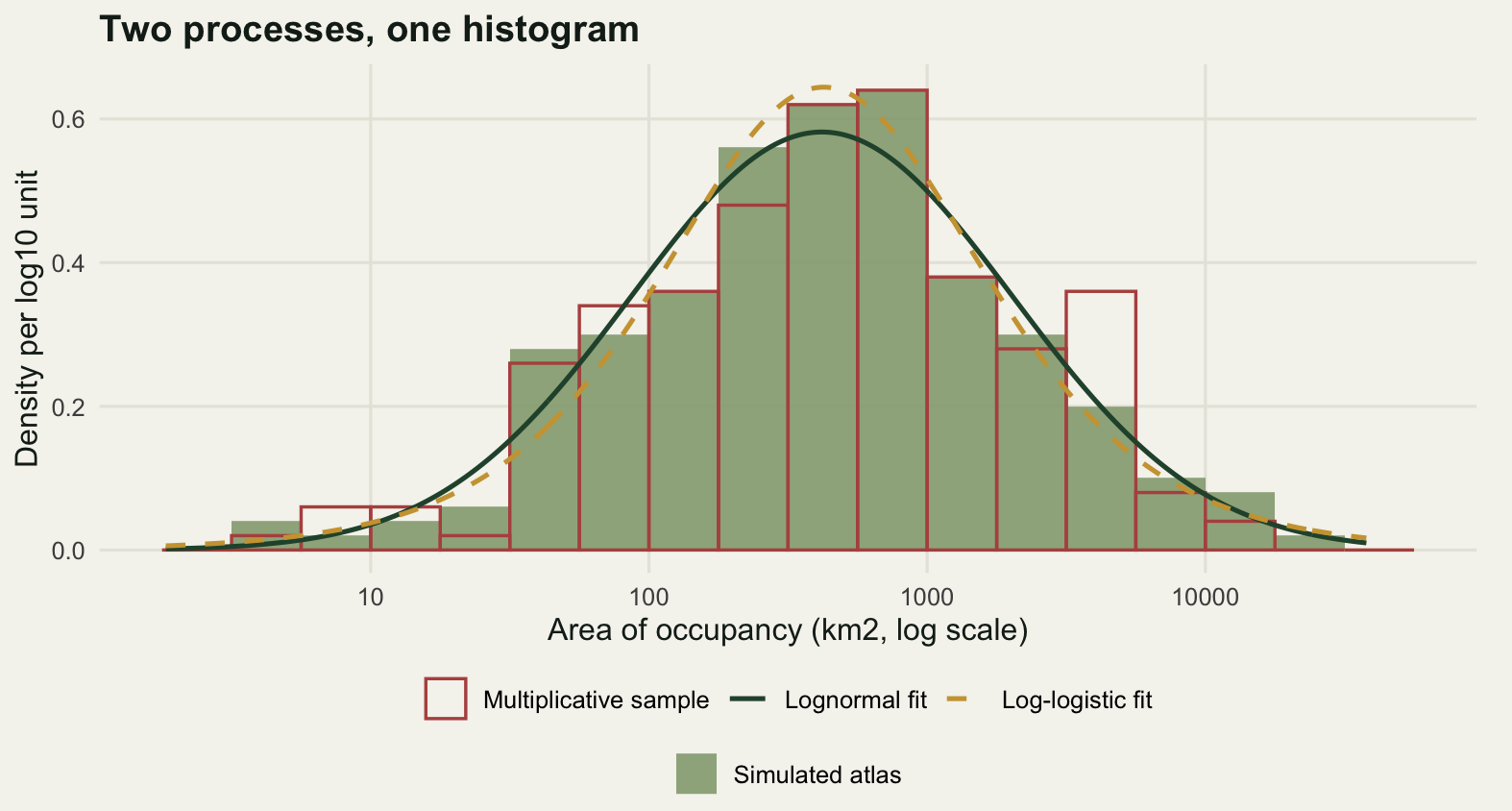
On the atlas the AIC gap between the lognormal and the log-logistic is 1.6104 units. That looks like a result until it is compared with the noise. Draw 200 species from a lognormal, so that the answer is known, and the median advantage the lognormal takes is 4.3150 units, with AIC picking the right family 87.50 per cent of the time. When the log-logistic is the truth it picks right 80.75 per cent of the time, 84.12 per cent across the two. On the sample size a regional atlas actually gives you the criterion is wrong about one time in six, and the separation observed here falls inside the spread of separations you see when the answer is known.
The outlined histogram is the other half of the argument. That sample was drawn from neither family: it is a product of six uniform draws, standardised on the log scale. It sits on top of the atlas histogram. The correlation between its sorted log values and normal quantiles is 0.9952, against 0.9973 for the atlas, so a lognormal describes a process that is not lognormal just as well as it describes the atlas, and it wins there too, by 5.8681 AIC units, on data that no lognormal produced. Fitting a lognormal to a range size distribution and reporting that it fits is not evidence about the mechanism that made the ranges. The shape is the signature of multiplication, not of any particular biology.
Grain
Now change one thing the analyst controls and nothing about the species. Aggregate the same occurrence records to grids of 2, 4, 8 and 16 km cells and recompute the area of occupancy at each. Area of occupancy always rises when the cell gets bigger, because the occupied cells fall in number more slowly than they grow in area. The rate at which it rises is the exponent of area of occupancy against cell area, and it varies between species.
grains <- c(1, 2, 4, 8)
side_km <- grains * cell_km
log_area <- log(side_km^2)

aoo_at <- function(k, b) {
  length(unique(((gx[k] - 1) %/% b) + ((gy[k] - 1) %/% b) * (nx / b))) *
    (b * cell_km)^2
}
A <- sapply(grains, function(b) vapply(occ, aoo_at, 1, b = b))
colnames(A) <- paste0(side_km, "km")

slope_of <- function(v) {
  sum((log_area - mean(log_area)) * (log(v) - mean(log(v)))) /
    sum((log_area - mean(log_area))^2)
}
expo <- apply(A, 1, slope_of)

contig <- vapply(occ, function(k) {
  o <- logical(n_cell)
  o[k] <- TRUE
  mean(o[pmin(k + 1, n_cell)] | o[pmax(k - 1, 1)] |
         o[pmin(k + nx, n_cell)] | o[pmax(k - nx, 1)])
}, 1)

sd_grain <- apply(log(A), 2, sd)
# what the box plot below actually draws, so the caption can name the right part
# of it: the box is the interquartile range, the whiskers the 1.5 IQR reach
iqr_grain <- apply(log10(A), 2, IQR)
whisk_grain <- apply(log10(A), 2, function(v) diff(range(boxplot.stats(v)$stats)))
thr <- apply(A, 2, function(v) c(at_or_below_2000 = sum(v <= 2000),
                                 at_or_below_500 = sum(v <= 500)))

print(round(apply(A, 2, median), 1))
2km 4km 8km 16km
442 1192 2336 4096 print(round(sd_grain, 4)) 2km 4km 8km 16km
1.5828 1.5623 1.4904 1.3167 print(round(rbind(interquartile_range = iqr_grain,
whisker_span = whisk_grain), 4)) 2km 4km 8km 16km
interquartile_range 0.8931 0.8675 0.8719 0.8270
whisker_span 3.3756 3.1337 2.9845 2.4065print(thr) 2km 4km 8km 16km
at_or_below_2000 166 130 92 55
at_or_below_500 107 57 31 4round(c(exponent_tight_species = expo[sp_tight],
exponent_loose_species = expo[sp_loose],
contiguity_tight = contig[sp_tight],
contiguity_loose = contig[sp_loose],
aoo_ratio_at_2km = pair_aoo_ratio,
aoo_ratio_at_16km = A[sp_loose, 4] / A[sp_tight, 4],
smallest_exponent = min(expo), largest_exponent = max(expo),
median_exponent = median(expo),
coarse_grid_cells = n_cell / 64,
widest_species_share_of_the_coarse_grid =
max(A[, 4]) / region_area), 4) exponent_tight_species exponent_loose_species
0.3617 0.6650
contiguity_tight contiguity_loose
0.8031 0.5467
aoo_ratio_at_2km aoo_ratio_at_16km.16km
1.1811 4.2222
smallest_exponent largest_exponent
0.2924 1.0000
median_exponent coarse_grid_cells
0.5631 256.0000
widest_species_share_of_the_coarse_grid
0.9961 The median species goes from 442 square kilometres at 2 km cells to 4096 at 16 km cells. The two species from the map start almost level: at 2 km cells the loosely packed one has 1.1811 times the area of occupancy of the tightly packed one. At 16 km cells it has 4.2222 times as much. Their exponents are 0.3617 and 0.6650.
Both lie between 0 and 1, and both limits are informative. A species whose occupied cells form one solid block loses cells exactly as fast as the cells gain area, so its area of occupancy does not change at all and its exponent is 0. A species whose occupied cells are so far apart that no two ever land in the same coarse cell keeps every cell it had, so its area of occupancy scales with the cell area and its exponent is 1. Every species sits between those, and where it sits is a statement about how its occurrences are arranged as much as about how large its range is.
The measurement backs that up. Contiguity here is the share of a species’ occupied cells that have at least one occupied neighbour to the north, south, east or west. Regress the exponent on contiguity and on log range size together and both matter, and both pull the exponent down. The gap between the two coefficients below does not rank them, because they are not on a common scale: contiguity is a proportion while log range size runs over several natural log units, so a step of one in each is a different size of step.
m_expo <- lm(expo ~ log(aoo) + contig)
cf <- coef(m_expo)
r2_expo <- summary(m_expo)$r.squared
rho_grain <- cor(A[, 1], A[, 4], method = "spearman")

r1 <- rank(-A[, 1], ties.method = "min")
r4 <- rank(-A[, 4], ties.method = "min")
riser <- which.max(r1 - r4)
gained <- r1[riser] - r4[riser]

round(c(intercept = cf[[1]], slope_on_log_aoo = cf[[2]],
        slope_on_contiguity = cf[[3]], r_squared = r2_expo,
        lowest_contiguity = min(contig), highest_contiguity = max(contig),
        spearman_2km_against_16km = rho_grain,
        biggest_riser = riser,
        its_rank_at_2km = r1[riser], its_rank_at_16km = r4[riser],
        places_gained = gained,
        its_contiguity = contig[riser], its_exponent = expo[riser],
        its_aoo_at_2km = A[riser, 1], its_aoo_at_16km = A[riser, 4]), 4)
intercept slope_on_log_aoo slope_on_contiguity
1.0200 -0.0374 -0.3814
r_squared lowest_contiguity highest_contiguity
0.7108 0.0000 1.0000
spearman_2km_against_16km biggest_riser its_rank_at_2km
0.9605 174.0000 127.0000
its_rank_at_16km places_gained its_contiguity
73.0000 54.0000 0.2273
its_exponent its_aoo_at_2km.2km its_aoo_at_16km.16km
0.8010 264.0000 7168.0000 box_df <- data.frame(
grain = factor(rep(colnames(A), each = n_sp), levels = colnames(A)),
laoo = as.numeric(log10(A)))
trace_lab <- c("Tightly packed species", "Loosely packed species",
"Largest rank gain")
trace_df <- data.frame(
grain = factor(rep(colnames(A), 3), levels = colnames(A)),
laoo = log10(c(A[sp_tight, ], A[sp_loose, ], A[riser, ])),
who = factor(rep(trace_lab, each = length(grains)), levels = trace_lab))
ggplot() +
geom_boxplot(data = box_df, aes(grain, laoo), fill = te_pal$line,
colour = te_pal$ink, width = 0.5,
outlier.size = 0.9, outlier.colour = te_pal$ink) +
geom_line(data = trace_df, aes(grain, laoo, colour = who, group = who),
linewidth = 0.9) +
geom_point(data = trace_df, aes(grain, laoo, colour = who), size = 2.6) +
scale_colour_manual(values = c(te_pal$forest, te_pal$clay, te_pal$gold),
name = NULL) +
labs(x = "Grid cell side (km)", y = "log10 area of occupancy (km2)",
title = "Coarsening the grid reorders the species") +
theme_te() +
theme(plot.margin = margin(6, 14, 6, 6))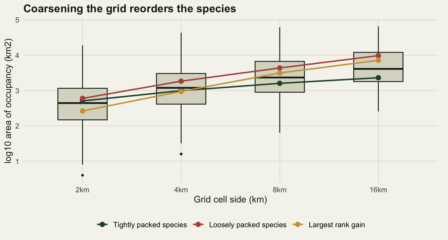
The rank correlation between the finest and the coarsest grid is 0.9605, which sounds like agreement and is not. Species 174 sits at position 127 in the ranking by area of occupancy on the 2 km grid and at position 73 on the 16 km grid, a gain of 54 places out of 200. Its contiguity is 0.2273, low for the atlas: it holds scattered single cells, so fewer of them merge under aggregation than for almost any other species in the atlas, and its exponent is 0.8010 against a median across the atlas of 0.5631. Nothing about the species changed. The grid changed.
The consequence for an assessment is arithmetic. On the 2 km grid, 166 of the 200 species have an area of occupancy at or below the 2000 square kilometre Vulnerable threshold and 107 are at or below the 500 square kilometre Endangered threshold. Move to 4 km cells and those counts become 130 and 57. On 16 km cells they are 55 and 4. Same records, same species, four different red lists. This is why the IUCN guidelines name a resolution instead of leaving it open, and why an area of occupancy quoted without its grain is not a quantity at all.
The standard deviation of log area of occupancy falls from 1.5828 at 2 km to 1.3167 at 16 km, so the distribution does narrow as the grain coarsens. Part of that narrowing is a ceiling rather than a compression: the 16 km grid holds only 256 cells in total, and the widest species already fills 99.61 per cent of them.
Effort
An atlas cell is occupied in the data if somebody recorded the species there. Range size estimated from records is therefore a function of how many records the species has, and the direction of that dependence is fixed by an inequality rather than by an assumption. A subset of the occupied cells cannot contain more cells than the full set, and the convex hull of a subset of the points cannot be larger than the hull of all of them. Both estimates are bounded above by the truth. Every error runs the same way, and it makes the species look narrower ranged and so more threatened.
The first measurement is a controlled sweep: give every species the same number of records, drawn with replacement from its occupied cells, and recompute both areas.
set.seed(9312)

levels_rec <- c(5, 10, 20, 40, 80, 160, 320)
qa <- quantile(aoo, c(0.25, 0.75))

sweep_one <- function(L) {
  ra <- numeric(n_sp)
  re <- rep(NA_real_, n_sp)
  for (i in seq_len(n_sp)) {
    k <- occ[[i]]
    u <- unique(k[sample.int(length(k), L, replace = TRUE)])
    ra[i] <- length(u) * cell_area
    re[i] <- hull_area(gx[u] * cell_km, gy[u] * cell_km)
  }
  small <- aoo <= qa[1]
  big <- aoo >= qa[2]
  c(records = L,
    aoo_all = mean(ra / aoo), eoo_all = mean(re / eoo, na.rm = TRUE),
    aoo_small = mean((ra / aoo)[small]),
    eoo_small = mean((re / eoo)[small], na.rm = TRUE),
    aoo_big = mean((ra / aoo)[big]),
    eoo_big = mean((re / eoo)[big], na.rm = TRUE),
    eoo_undefined = sum(is.na(re) & !is.na(eoo)))
}
sw <- t(vapply(levels_rec, sweep_one, numeric(8)))
rownames(sw) <- paste0(levels_rec, " records")
print(round(sw, 4))
records aoo_all eoo_all aoo_small eoo_small aoo_big eoo_big
5 records 5 0.1138 0.1663 0.3387 0.2736 0.0082 0.1197
10 records 10 0.1897 0.3462 0.5336 0.5811 0.0162 0.2512
20 records 20 0.2869 0.5028 0.7314 0.7826 0.0319 0.3946
40 records 40 0.4014 0.6548 0.8657 0.8853 0.0634 0.5340
80 records 80 0.5446 0.8178 0.9713 0.9936 0.1209 0.6947
160 records 160 0.6832 0.9003 0.9984 1.0000 0.2209 0.7956
320 records 320 0.8035 0.9592 1.0000 1.0000 0.3799 0.8861
eoo_undefined
5 records 3
10 records 0
20 records 0
40 records 0
80 records 0
160 records 0
320 records 0grp <- c("All species", "Narrowest quarter", "Widest quarter")
eff_df <- data.frame(
records = log2(rep(sw[, "records"], 6)),
ratio = c(sw[, "aoo_all"], sw[, "aoo_small"], sw[, "aoo_big"],
sw[, "eoo_all"], sw[, "eoo_small"], sw[, "eoo_big"]),
measure = factor(rep(c("Area of occupancy", "Extent of occurrence"),
each = 3 * nrow(sw)),
levels = c("Area of occupancy", "Extent of occurrence")),
panel = factor(rep(rep(grp, each = nrow(sw)), 2), levels = grp))
truth_lab <- data.frame(records = log2(min(levels_rec)), ratio = 1.045,
panel = factor(grp[1], levels = grp))
ggplot(eff_df, aes(records, ratio, colour = measure, shape = measure,
linetype = measure)) +
geom_hline(yintercept = 1, linetype = 2, colour = te_pal$ink,
linewidth = 0.5) +
geom_text(data = truth_lab, aes(records, ratio), label = "truth",
inherit.aes = FALSE, hjust = 0, vjust = 0, size = 3.1,
colour = te_pal$ink) +
geom_line(linewidth = 0.9) +
geom_point(size = 2.4) +
facet_wrap(~panel) +
scale_colour_manual(values = c(te_pal$forest, te_pal$gold), name = NULL) +
scale_shape_manual(values = c(16, 17), name = NULL) +
scale_linetype_manual(values = c(1, 2), name = NULL) +
scale_x_continuous(breaks = log2(levels_rec), labels = levels_rec) +
scale_y_continuous(limits = c(0, 1.1), breaks = seq(0, 1, 0.25)) +
labs(x = "Records per species", y = "Estimated over true range size",
title = "Both measures are biased down, at different rates") +
theme_te() +
theme(strip.text = element_text(colour = te_pal$ink, face = "bold",
size = 9),
plot.margin = margin(6, 14, 6, 6))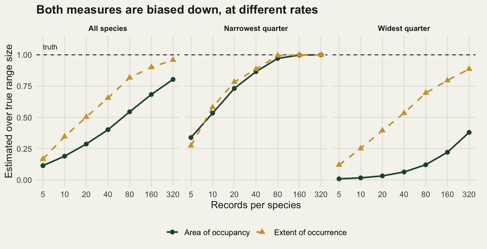
At 20 records per species the mean estimated area of occupancy is 0.2869 of the truth and the mean estimated extent of occurrence is 0.5028. At 320 records they are 0.8035 and 0.9592. The gap between the two measures is geometry. A hull is decided by a handful of points near the edge of the range, so a few records place it approximately; an area of occupancy needs a record in every occupied cell and there is no shortcut. In the widest quarter of the distribution, 320 records recover 0.3799 of the true area of occupancy. A widespread species assessed on records alone would be reported at under half its area.
That is a sweep at constant effort, and constant effort is not what atlases have. Records accumulate faster for species that are both widespread and locally common, which is the abundance-occupancy relationship doing its work, so the expected record count here is set proportional to the number of occupied cells raised to the power 1.25, with lognormal noise on top. The exponent above one is what thins the small-range end: a narrow ranged species gets fewer records per occupied cell than a widespread one, not merely fewer records.
set.seed(2026)

lambda <- 0.20 * nocc^1.25 * exp(rnorm(n_sp, 0, 0.6))
n_rec <- rpois(n_sp, lambda)

est_a <- numeric(n_sp)
est_e <- rep(NA_real_, n_sp)
for (i in seq_len(n_sp)) {
  if (n_rec[i] == 0) next
  k <- occ[[i]]
  u <- unique(k[sample.int(length(k), n_rec[i], replace = TRUE)])
  est_a[i] <- length(u) * cell_area
  est_e[i] <- hull_area(gx[u] * cell_km, gy[u] * cell_km)
}
qtl <- cut(aoo, quantile(aoo, 0:4 / 4), include.lowest = TRUE,
           labels = c("Q1 narrowest", "Q2", "Q3", "Q4 widest"))
by_q <- rbind(
  median_records = tapply(n_rec, qtl, median),
  records_per_occupied_cell = round(tapply(n_rec / nocc, qtl, median), 4),
  mean_aoo_ratio = round(tapply(est_a / aoo, qtl, mean), 4),
  mean_eoo_ratio = round(tapply(est_e / eoo, qtl,
                                function(z) mean(z, na.rm = TRUE)), 4))
print(by_q)
Q1 narrowest Q2 Q3 Q4 widest
median_records 6.0000 48.0000 121.0000 592.0000
records_per_occupied_cell 0.3750 0.5870 0.7318 0.9508
mean_aoo_ratio 0.3405 0.5052 0.5112 0.6160
mean_eoo_ratio 0.5322 0.6865 0.7947 0.9181pushed_2000 <- sum(aoo > 2000 & est_a <= 2000)
pushed_500 <- sum(aoo > 500 & est_a <= 500)
lost_hull <- sum(is.na(est_e))
round(c(total_records = sum(n_rec), fewest_records = min(n_rec),
median_records = median(n_rec), most_records = max(n_rec),
species_with_no_records = sum(n_rec == 0),
eoo_undefined_after_thinning = lost_hull,
true_at_or_below_2000 = sum(aoo <= 2000),
estimated_at_or_below_2000 = sum(est_a <= 2000),
true_at_or_below_500 = sum(aoo <= 500),
estimated_at_or_below_500 = sum(est_a <= 500),
pushed_below_2000_by_effort = pushed_2000,
pushed_above_2000_by_effort = sum(aoo <= 2000 & est_a > 2000),
pushed_below_500_by_effort = pushed_500,
pushed_above_500_by_effort = sum(aoo <= 500 & est_a > 500)), 4) total_records fewest_records
124929.0 0.0
median_records most_records
73.5 38641.0
species_with_no_records eoo_undefined_after_thinning
5.0 14.0
true_at_or_below_2000 estimated_at_or_below_2000
166.0 182.0
true_at_or_below_500 estimated_at_or_below_500
107.0 141.0
pushed_below_2000_by_effort pushed_above_2000_by_effort
16.0 0.0
pushed_below_500_by_effort pushed_above_500_by_effort
34.0 0.0 The atlas holds 124929 records after that thinning, which is a plausible size for a thirty year regional dataset, and the effort is distributed the way atlas effort is distributed. The widest quarter of species has a median of 592 records and the narrowest quarter a median of 6. Per occupied cell that is 0.9508 records against 0.3750, so the narrow ranged species are sampled at less than half the intensity of the wide ranged ones. The mean ratio of estimated to true area of occupancy is 0.3405 in the narrowest quarter and 0.6160 in the widest, and for extent of occurrence 0.5322 against 0.9181. Both measures are worst where the thresholds are.
The bias runs one way and the counts say what that costs. 166 species truly sit at or below the Vulnerable threshold and 182 appear to: 16 species are pushed across the line by effort and 0 are pushed back the other way. At the Endangered threshold the true count is 107 and the estimated count is 141, 34 species moved in and none moved out. 14 species end up with fewer than three distinct cells recorded, which leaves their extent of occurrence undefined rather than small. In practice an assessor faced with that writes down a small number rather than a missing one, and the error runs in the same direction again.
EOO against AOO
The two measures correlate well enough across the atlas to look interchangeable. They are not.
ok <- !is.na(eoo)
ratio <- eoo / aoo
dense <- which(ratio == min(ratio, na.rm = TRUE))
sparse <- which(ratio == max(ratio, na.rm = TRUE))
r_log <- cor(log(aoo[ok]), log(eoo[ok]))
rho <- cor(aoo[ok], eoo[ok], method = "spearman")
q_lo <- quantile(ratio, 0.05, na.rm = TRUE)
q_hi <- quantile(ratio, 0.95, na.rm = TRUE)

round(c(species_compared = sum(ok),
        pearson_on_logs = r_log, spearman = rho,
        median_eoo_over_aoo = median(ratio, na.rm = TRUE),
        eoo_over_aoo_5th_percentile = q_lo,
        eoo_over_aoo_95th_percentile = q_hi,
        spread_of_that_ratio = q_hi / q_lo,
        densest_species = dense, densest_cells = nocc[dense],
        densest_aoo_km2 = aoo[dense], densest_eoo_km2 = eoo[dense],
        sparsest_species = sparse, sparsest_cells = nocc[sparse],
        sparsest_aoo_km2 = aoo[sparse], sparsest_eoo_km2 = eoo[sparse],
        sparsest_eoo_over_aoo = ratio[sparse]), 4)
species_compared pearson_on_logs
197.0000 0.9132
spearman median_eoo_over_aoo
0.9194 7.6151
eoo_over_aoo_5th_percentile.5% eoo_over_aoo_95th_percentile.95%
1.6063 40.2857
spread_of_that_ratio.95% densest_species
25.0790 31.0000
densest_cells densest_aoo_km2
3.0000 12.0000
densest_eoo_km2 sparsest_species
2.0000 52.0000
sparsest_cells sparsest_aoo_km2
76.0000 304.0000
sparsest_eoo_km2 sparsest_eoo_over_aoo
31156.0000 102.4868 The correlation of the logs is 0.9132 and the rank correlation is 0.9194, which would be written up as strong agreement in most papers. The ratio between the two measures tells the other story. The middle species has an extent of occurrence 7.6151 times its area of occupancy, but the ratio runs from 1.6063 at the fifth percentile to 40.2857 at the ninety-fifth, a spread of 25.0790. Knowing one measure pins the other only to within that factor.
The two extremes show what the ratio is made of. Species 31 occupies 3 cells side by side. Its area of occupancy is 12 square kilometres and the hull drawn round the 3 cell centres is 2 square kilometres, so its extent of occurrence comes out smaller than its area of occupancy. That is arithmetically possible and biologically meaningless: the hull is drawn round points, and the cells those points stand for have width. The IUCN guidance says as much, and an extent of occurrence should never be reported below the area of occupancy.
Species 52 goes the other way. It occupies 76 cells for an area of occupancy of 304 square kilometres, and its convex hull covers 31156 square kilometres, which is 102.4868 times as much, because a few outlying populations drag the polygon across half the region. On area of occupancy it is a restricted species. On extent of occurrence it is a regional generalist. Both numbers are right and they answer different questions: how much ground the species is on, and how far apart the pieces of it are. The loosely packed species from the map does the same thing less extremely, at 60.4733 times.
A conservation plan that weights species by range size has to pick one and say which. Checking a prioritisation uses a range size weighted target and measures what the weighting does to the reserve network that comes out; the point here sits upstream of that, which is that the weight itself moves by more than an order of magnitude depending on a definition.
The honest limit
Everything above rests on a truth column and a real atlas does not have one. There is no operation you can perform on a set of records that returns the true area of occupancy, because the cells with no record are of two kinds and the data do not separate them: cells the species is absent from, and cells nobody visited. Correcting for that is the same job as correcting reporting rates for effort drift, and it needs the list lengths or the visit records that most historical atlases never kept.
The second limit is in the tail, and it can be measured. The small-range end is where the assessments happen and it is also where the fewest species inform the shape. Resample the 200 species with replacement, refit the lognormal each time, and read off the spread.
set.seed(5150)

n_boot <- 2000
boot <- t(replicate(n_boot, {
  s <- sample(n_sp, n_sp, replace = TRUE)
  yy <- y[s]
  m <- mean(yy)
  v <- sqrt(mean((yy - m)^2))
  c(v, exp(qnorm(0.05, m, v)), mean(exp(yy) <= 2000), mean(exp(yy) <= 500))
}))

q05 <- exp(qnorm(0.05, mu, sigma))
ci <- apply(boot, 2, quantile, c(0.025, 0.975))
n_in_tail <- sum(aoo <= q05)

round(c(bootstrap_replicates = n_boot,
        sigma = sigma, sigma_low = ci[1, 1], sigma_high = ci[2, 1],
        fitted_5th_percentile_km2 = q05,
        fitted_5th_percentile_low = ci[1, 2],
        fitted_5th_percentile_high = ci[2, 2],
        width_as_a_ratio = ci[2, 2] / ci[1, 2],
        species_at_or_below_the_fitted_5th_percentile = n_in_tail,
        share_at_or_below_2000 = mean(aoo <= 2000),
        share_at_or_below_2000_low = ci[1, 3],
        share_at_or_below_2000_high = ci[2, 3],
        share_at_or_below_500 = mean(aoo <= 500),
        share_at_or_below_500_low = ci[1, 4],
        share_at_or_below_500_high = ci[2, 4]), 4)
bootstrap_replicates
2000.0000
sigma
1.5789
sigma_low.2.5%
1.4135
sigma_high.97.5%
1.7402
fitted_5th_percentile_km2
31.1776
fitted_5th_percentile_low.2.5%
21.8586
fitted_5th_percentile_high.97.5%
45.0638
width_as_a_ratio.97.5%
2.0616
species_at_or_below_the_fitted_5th_percentile
8.0000
share_at_or_below_2000
0.8300
share_at_or_below_2000_low.2.5%
0.7750
share_at_or_below_2000_high.97.5%
0.8800
share_at_or_below_500
0.5350
share_at_or_below_500_low.2.5%
0.4650
share_at_or_below_500_high.97.5%
0.6050 The fitted standard deviation on the log scale is 1.5789 with a bootstrap interval from 1.4135 to 1.7402, tight enough to work with. The fifth percentile of the fitted distribution, which is the sort of quantity a red list leans on, is 31.1776 square kilometres with an interval from 21.8586 to 45.0638: a factor of 2.0616 from one end to the other, out of the same 200 species. Only 8 species lie at or below that percentile, but the fit does not read it off those 8 alone: it reads it off the mean and the standard deviation of all 200 logged values. Much of the width comes from the standard deviation, because a fifth percentile is placed by it as well as by the mean, while the fitted median would use the mean alone. The share of species at or below the Vulnerable threshold is steadier, 0.8300 with an interval from 0.7750 to 0.8800, because most of the distribution contributes to it. The further into the tail the question goes, the less the atlas has to say.
The third limit is the generator. Ranges here are a smooth environmental preference plus a geographic extent plus scatter, and real ranges have structure this does not reproduce: hard coastlines, elevational bands, historical absences from perfectly suitable habitat, and boundaries that fall outside the study region so that the atlas holds a slice of a range rather than a range. That last one is systematic rather than random. Every species whose distribution crosses the edge of the region has its area of occupancy truncated at the border, the truncation is worse for the widespread species, and it flattens the right tail of the distribution in a way none of the measurements here would detect.
Where to go next
If the records come from a public aggregator rather than a structured atlas, the cleaning comes first. Cleaning GBIF occurrence data covers the coordinate errors and duplicated records that inflate both measures before either can be computed, and a misplaced record inflates an extent of occurrence far more efficiently than it inflates an area of occupancy: one point in the wrong country moves the hull and adds a single cell. The spatial bias in those records is measured in sampling bias in presence-only models, which is the effort problem from the modelling side.
For the pattern-checking habit that the second section is an instance of, checking a macroecological pattern works the general case: a strong shape, a plausible mechanism, and the question of what would have to be true for the shape to count as evidence. And if the atlas cells are going to become a richness map rather than a set of per-species ranges, mapping species richness with sf is the next step, with the same grain warning attached to it.
References
Gaston KJ 1996 Trends in Ecology and Evolution 11(5):197-201 (10.1016/0169-5347(96)10027-6)
Gaston KJ, Fuller RA 2009 Journal of Applied Ecology 46(1):1-9 (10.1111/j.1365-2664.2008.01596.x)
Kunin WE 1998 Science 281(5382):1513-1515 (10.1126/science.281.5382.1513)
Hartley S, Kunin WE 2003 Conservation Biology 17(6):1559-1570 (10.1111/j.1523-1739.2003.00015.x)
Hurlbert AH, Jetz W 2007 Proceedings of the National Academy of Sciences 104(33):13384-13389 (10.1073/pnas.0704469104)
Isaac NJB, Pocock MJO 2015 Biological Journal of the Linnean Society 115(3):522-531 (10.1111/bij.12532)