Sampling bias in presence-only models

Survey effort thins presence-only records: measuring how much sampling bias an effort covariate, target-group background and spatial thinning remove in R.

A presence-only dataset is a sample of a species taken by people. Every record needed somebody to be in the right place, to look, to identify, and to submit. What arrives in the database is the species thinned by the pattern of human attention, and that pattern is rarely flat: roads, reserve boundaries, university towns and holiday seasons all leave their shape in the point cloud.

The standard remedies are known: put an effort covariate in the model, draw the background from records of similarly surveyed species, or thin the occurrences in space. The tutorial on choosing pseudo-absences and background points sets out what each one is for. What it does not do, and what almost nothing in the applied literature does, is measure how much of the bias each one actually removes, and under what condition each one fails. That is the gap here.

The question is deliberately narrow: what can be done with presence-only records alone? A separate route exists, which is to collect a structured survey and fit the two datasets jointly, and it gets its own tutorial at the end of this one. Here there is no second dataset. There are records, an environmental layer, and whatever side information about effort can be scraped together.

The fitting throughout is presence-versus-background logistic regression, which recovers the log ratio of the density of records to the density of background points; the point process reading of MaxEnt explains why that ratio is the right target, and it is taken as given here. The simulation controls one thing carefully: the correlation between survey effort and the environmental covariate. That correlation, and not the severity of the bias, decides whether any remedy helps.

library(ggplot2)

te_pal <- list(forest = "#275139", green = "#2f8f63", sage = "#93a87f",
               clay = "#b5534e", gold = "#cda23f", line = "#dad9ca",
               ink = "#16241d", paper = "#f5f4ee")

theme_te <- function() {
  theme_minimal(base_size = 12) +
    theme(panel.grid.minor = element_blank(),
          panel.grid.major = element_line(colour = "#e7e6dc"),
          plot.background = element_rect(fill = "#f5f4ee", colour = NA),
          panel.background = element_rect(fill = "#f5f4ee", colour = NA),
          plot.title = element_text(face = "bold", colour = te_pal$ink),
          axis.title = element_text(colour = "#2c3a31"))
}

A species, a survey, and the records that survive both

The grid is 60 by 60 cells. Two smooth surfaces live on it: an environmental covariate, drawn at a coarse spatial scale, and an accessibility surface, drawn at a finer one. Individuals of the species arrive as a Poisson process whose log intensity is a linear function of the environment with slope 1.2. Each individual is then recorded with a probability that rises log-linearly with accessibility, slope 1.0. The thinning is severe at the difficult end of the gradient and complete at the easiest cell.

The effort surface used in a given run is a mixture of the accessibility surface and the environment, with the mixing weight set so that their correlation takes whatever value the run needs. That gives a dial from zero to strong.

One design decision is worth stating first, because it matters more than it looks. Twelve accessibility surfaces are drawn, all orthogonalised against the environment so that the sample correlation is zero to machine precision. For each, the asymptotic slope a naive fit would return is computed directly, by maximising the population logistic likelihood over the grid rather than by simulating records. Those twelve numbers are not all 1.2. The surface used for the rest of the post is the one closest to neutral; the worst of the twelve comes back in a moment.

set.seed(20260816)
nx <- 60
n_cell <- nx * nx
gx <- rep(seq_len(nx), times = nx)
gy <- rep(seq_len(nx), each = nx)
b_env <- 1.2
g_eff <- 1.0
lam0 <- 1.1
n_bg <- 10000
n_cand <- 12

zstd <- function(v) (v - mean(v)) / sd(v)
smooth_field <- function(ux, uy, n_basis, f_max) {
  out <- numeric(length(ux))
  for (k in seq_len(n_basis)) {
    wx <- sample(seq_len(f_max), 1); wy <- sample(seq_len(f_max), 1)
    out <- out + rnorm(1) * cos(2 * pi * (wx * ux + wy * uy) / nx + runif(1, 0, 2 * pi))
  }
  zstd(out)
}
env <- smooth_field(gx, gy, 3, 2)

softplus <- function(z) ifelse(z > 30, z, log1p(exp(z)))
pop_slope <- function(effv, ratio) {
  w1 <- exp(b_env * env + g_eff * effv); w1 <- ratio * w1 / sum(w1)
  w0 <- rep(1 / n_cell, n_cell)
  nll <- function(par) {
    eta <- par[1] + par[2] * env
    -sum(w1 * eta - (w1 + w0) * softplus(eta))
  }
  optim(c(-2, 1), nll, method = "BFGS")$par[2]
}

set.seed(313)
cand_list <- replicate(n_cand, zstd(residuals(lm(smooth_field(gx, gy, 8, 5) ~ env))),
                       simplify = FALSE)
cand_slope <- vapply(cand_list, pop_slope, numeric(1), ratio = 0.15)
acc_perp <- cand_list[[which.min(abs(cand_slope - b_env))]]
acc_bad <- cand_list[[which.max(abs(cand_slope - b_env))]]
cat(sprintf("candidate access surfaces %d; all correlations with environment below %.1e\n",
            n_cand, max(abs(vapply(cand_list, function(v) cor(v, env), numeric(1))))))

candidate access surfaces 12; all correlations with environment below 4.6e-16

cat(sprintf("asymptotic naive slope over the candidates: %.3f to %.3f (truth %.1f)\n",
            min(cand_slope), max(cand_slope), b_env))

asymptotic naive slope over the candidates: 0.900 to 1.626 (truth 1.2)

cat(sprintf("chosen surface %.4f, worst surface %.4f\n",
            pop_slope(acc_perp, 0.15), pop_slope(acc_bad, 0.15)))

chosen surface 1.2126, worst surface 1.6264

make_effort <- function(rho) zstd(rho * env + sqrt(1 - rho^2) * acc_perp)
draw_records <- function(effv) {
  det_p <- exp(g_eff * (effv - max(effv)))
  rep(seq_len(n_cell), rbinom(n_cell, rpois(n_cell, lam0 * exp(b_env * env)), det_p))
}
uni_bg <- function() sample(seq_len(n_cell), n_bg, replace = TRUE)
fit_pb <- function(rc, bc, form, covs) {
  dd <- cbind(data.frame(pres = c(rep(1, length(rc)), rep(0, length(bc)))),
              covs[c(rc, bc), , drop = FALSE])
  glm(form, data = dd, family = binomial())
}

eff_ref <- make_effort(0.6)
covs_ref <- data.frame(env = env, eff = eff_ref)
det_ref <- exp(g_eff * (eff_ref - max(eff_ref)))
n_ind_ref <- rpois(n_cell, lam0 * exp(b_env * env))
rec_ref <- rbinom(n_cell, n_ind_ref, det_ref)
cat(sprintf("grid %d by %d = %d cells; true slopes environment %.1f effort %.1f\n",
            nx, nx, n_cell, b_env, g_eff))

grid 60 by 60 = 3600 cells; true slopes environment 1.2 effort 1.0

cat(sprintf("individuals %d, records %d, share recorded %.3f, cells holding a record %d\n",
            sum(n_ind_ref), sum(rec_ref), sum(rec_ref) / sum(n_ind_ref), sum(rec_ref > 0)))

individuals 7591, records 1266, share recorded 0.167, cells holding a record 663

cat(sprintf("detection probability %.4f to %.4f, a ratio of %.0f; correlation %.3f\n",
            min(det_ref), max(det_ref), max(det_ref) / min(det_ref), cor(env, eff_ref)))

detection probability 0.0049 to 1.0000, a ratio of 202; correlation 0.600

cat(sprintf("background points per fit %d; records per occupied cell %.2f; busiest cell %d\n",
            n_bg, sum(rec_ref) / sum(rec_ref > 0), max(rec_ref)))

background points per fit 10000; records per occupied cell 1.91; busiest cell 18

At an effort-environment correlation of 0.6 the simulated survey turns 7591 individuals into 1266 records, so 16.7 per cent of the population left a trace, and the detection probability runs from 0.0049 in the least visited cell to 1 in the most visited, a ratio of 202. That is a heavier thinning than most real datasets suffer, and it is the situation the rest of the post has to survive.

rank01 <- function(v) (rank(v) - 0.5) / length(v)
lay_lv <- c("environment", "survey effort", "expected record density")
d_land <- data.frame(x = rep(gx, 3), y = rep(gy, 3),
  layer = factor(rep(lay_lv, each = n_cell), levels = c(lay_lv, "records received")),
  v = c(rank01(env), rank01(eff_ref), rank01(exp(b_env * env) * det_ref)))
d_pts <- data.frame(
  x = gx[rep(seq_len(n_cell), rec_ref)] + runif(sum(rec_ref), -0.4, 0.4),
  y = gy[rep(seq_len(n_cell), rec_ref)] + runif(sum(rec_ref), -0.4, 0.4),
  layer = factor("records received", levels = c(lay_lv, "records received")))
p_land <- ggplot(d_land, aes(x, y)) +
  geom_raster(aes(fill = v)) +
  geom_point(data = d_pts, colour = te_pal$forest, size = 0.45, alpha = 0.55) +
  facet_wrap(~layer, nrow = 2) +
  scale_fill_gradientn(colours = c(te_pal$paper, te_pal$sage, te_pal$green, te_pal$forest),
                       breaks = c(0.1, 0.5, 0.9), labels = c("low", "middle", "high")) +
  coord_equal(expand = FALSE, xlim = c(0.5, nx + 0.5), ylim = c(0.5, nx + 0.5)) +
  labs(title = "Effort decides which part of the species is recorded",
       x = NULL, y = NULL, fill = NULL) +
  theme_te() +
  theme(axis.text = element_blank(), panel.grid.major = element_blank(),
        legend.position = "bottom", legend.key.height = unit(0.3, "cm"),
        legend.key.width = unit(1.1, "cm"))
print(p_land)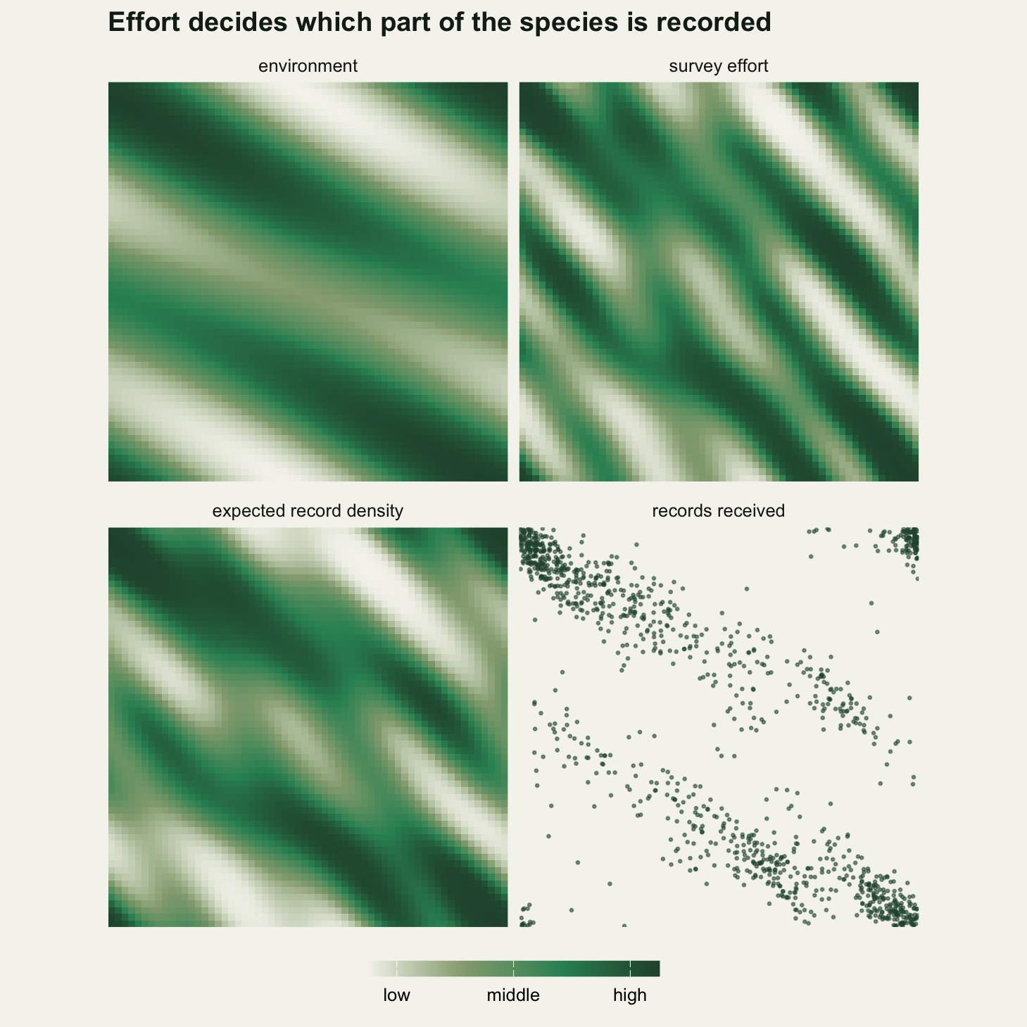

Figure 1: The two surfaces that generate the data, the record density they imply, and one realised set of records. Each raster panel is shaded by within-panel rank.

What the naive fit recovers, and when it is right

The loop below fits all four estimators at once, at five effort-environment correlations, with 25 replicate datasets at each. Later sections read off their own columns; this one reads the naive column, which is a plain fit of the environment against a uniformly drawn background.

The naive column also gets a check that costs nothing: for each correlation, pop_slope returns the slope the naive fit converges to as the dataset grows, computed by maximising the population likelihood over the grid rather than by simulating anything. If the simulated averages and the asymptotic values agree, both are probably right.

rho_seq <- c(0, 0.2, 0.4, 0.6, 0.8)
n_rep <- 25
set.seed(4242)
sweep_rows <- NULL
for (rh in rho_seq) {
  effv <- make_effort(rh)
  wt <- exp(g_eff * effv)
  covs <- data.frame(env = env, eff = effv)
  acc <- matrix(0, n_rep, 8)
  for (r in seq_len(n_rep)) {
    rc <- draw_records(effv); bc <- uni_bg()
    tg <- sample(seq_len(n_cell), n_bg, replace = TRUE, prob = wt)
    m1 <- fit_pb(rc, bc, pres ~ env, covs)
    m2 <- fit_pb(rc, bc, pres ~ env + eff, covs)
    m3 <- fit_pb(rc, tg, pres ~ env, covs)
    m4 <- fit_pb(unique(rc), bc, pres ~ env, covs)
    acc[r, ] <- c(coef(m1)[2], coef(m2)[2], coef(m3)[2], coef(m4)[2], coef(m2)[3],
                  length(rc), length(unique(rc)), summary(m1)$coefficients[2, 2])
  }
  sweep_rows <- rbind(sweep_rows, data.frame(rho = rh,
    naive = mean(acc[, 1]), effort = mean(acc[, 2]), tgb = mean(acc[, 3]),
    thinned = mean(acc[, 4]), eff_slope = mean(acc[, 5]),
    n_rec = mean(acc[, 6]), n_thin = mean(acc[, 7]),
    sd_naive = sd(acc[, 1]), sd_effort = sd(acc[, 2]), sd_tgb = sd(acc[, 3]),
    sd_thin = sd(acc[, 4])))
}
sweep_rows$asym_naive <- vapply(rho_seq, function(rh) pop_slope(make_effort(rh), 0.15), numeric(1))
print(round(sweep_rows[, c("rho", "n_rec", "naive", "asym_naive", "effort",
                           "eff_slope", "tgb", "thinned")], 3))

  rho   n_rec naive asym_naive effort eff_slope   tgb thinned
1 0.0 1299.52 1.202      1.213  1.189     1.011 1.188   0.837
2 0.2 1434.88 1.424      1.422  1.200     0.991 1.200   0.975
3 0.4 1329.96 1.642      1.634  1.208     0.993 1.200   1.140
4 0.6 1364.64 1.835      1.840  1.192     1.004 1.202   1.272
5 0.8 1551.72 2.034      2.033  1.219     0.980 1.198   1.404

cat(sprintf("correlations %d, replicate datasets each %d, background points %d\n",
            length(rho_seq), n_rep, n_bg))

correlations 5, replicate datasets each 25, background points 10000

cat(sprintf("naive error at zero correlation %.1f per cent; at 0.8 %.1f per cent\n",
            100 * (sweep_rows$naive[1] / b_env - 1), 100 * (sweep_rows$naive[5] / b_env - 1)))

naive error at zero correlation 0.1 per cent; at 0.8 69.5 per cent

cat(sprintf("largest gap between simulated and asymptotic naive slope %.3f\n",
            max(abs(sweep_rows$naive - sweep_rows$asym_naive))))

largest gap between simulated and asymptotic naive slope 0.011

The first row is the one to sit with. At zero correlation between effort and environment, the naive fit returns 1.202 against a truth of 1.2, an error of 0.1 per cent, and it does so on data where five individuals in six were never recorded and the least visited cell was surveyed 202 times less thoroughly than the best. Heavy sampling bias does not by itself bias the environmental slope. This is the part most discussions of the problem get wrong: they treat the severity of the thinning as the thing to worry about, when what matters is whether the thinning lines up with the covariate.

Once it does line up, the drift is fast and close to linear in the correlation: 1.424, 1.642, 1.835, and 2.034 at a correlation of 0.8, which is an error of 69.5 per cent. The asymptotic column never differs from the simulated one by more than 0.011, so this is a property of the estimator and not of the particular draws.

The catch is the wording. “Zero correlation” is a convenient shorthand for the real condition, which is that the expected value of the exponentiated effort surface should not trend across the environmental gradient. Correlation only measures the linear part of the association. The twelve candidate accessibility surfaces from the landscape chunk all had exactly zero correlation with the environment, and their asymptotic naive slopes ran from 0.900 to 1.626. The worst of them is worth a fit of its own.

set.seed(5150)
covs_bad <- data.frame(env = env, eff = acc_bad)
acc <- replicate(15, coef(fit_pb(draw_records(acc_bad), uni_bg(), pres ~ env, covs_bad))[2])
cat(sprintf("awkward surface: correlation %.1e, simulated naive slope %.3f, asymptotic %.3f\n",
            cor(acc_bad, env), mean(acc), pop_slope(acc_bad, 0.15)))

awkward surface: correlation 5.5e-17, simulated naive slope 1.634, asymptotic 1.626

cat(sprintf("neutral surface asymptotic %.3f; gap between the two surfaces %.3f\n",
            pop_slope(acc_perp, 0.15), pop_slope(acc_bad, 0.15) - pop_slope(acc_perp, 0.15)))

neutral surface asymptotic 1.213; gap between the two surfaces 0.414

An effort surface with a correlation of 6.9e-17 against the environment produces a naive slope of 1.634, an error of a third, while the surface chosen for the rest of the post produces 1.213 on the same species and the same generating model. The two differ by 0.414 in the recovered slope and by nothing at all in the diagnostic most people would run. Reporting the correlation between your effort proxy and your predictors is worth doing, but a value near zero is not a clean bill of health.

Effort as a covariate, and the prediction step people forget

The first remedy is to include the effort surface in the model. In the sweep table the effort column sits between 1.189 and 1.219 across the whole range of correlations, and the recovered effort slope stays near its true value of 1.0. As a way of recovering the environmental response it works, and it keeps working when the two surfaces are strongly aligned, which is exactly where the naive fit has fallen apart.

The coefficient is the easy half. What goes wrong in practice is the step after it. A fitted model with environment and effort in it predicts the density of records, so feeding the effort layer back into predict produces a map of where recorders will find the species, not a map of where the species is. The correct prediction holds effort at a constant, usually its mean, and lets only the environment vary. Both maps are computed below on ten replicate datasets, each normalised to mean one so they can be compared against the truth cell by cell.

set.seed(9091)
n_rep_p <- 10
lo <- which.min(eff_ref); hi <- which.max(eff_ref)
truth <- exp(b_env * env); truth <- truth / mean(truth)
pacc <- matrix(0, n_rep_p, 8)
for (r in seq_len(n_rep_p)) {
  rc <- draw_records(eff_ref); bc <- uni_bg()
  m_eff <- fit_pb(rc, bc, pres ~ env + eff, covs_ref)
  cf <- coef(m_eff)
  map_rec <- exp(cf[2] * env + cf[3] * eff_ref); map_rec <- map_rec / mean(map_rec)
  map_sp <- exp(cf[2] * env); map_sp <- map_sp / mean(map_sp)
  pacc[r, ] <- c(cf[2], cf[3], cor(map_rec, truth), cor(map_sp, truth),
                 map_rec[lo] / truth[lo], map_rec[hi] / truth[hi],
                 map_sp[lo] / truth[lo], map_sp[hi] / truth[hi])
}
pm <- colMeans(pacc)
cat(sprintf("replicate datasets %d, records in the last one %d\n", n_rep_p, length(rc)))

replicate datasets 10, records in the last one 1370

cat(sprintf("fitted slopes: environment %.3f, effort %.3f\n", pm[1], pm[2]))

fitted slopes: environment 1.184, effort 0.997

cat(sprintf("map of records vs truth: correlation %.3f; effort held constant %.4f\n",
            pm[3], pm[4]))

map of records vs truth: correlation 0.681; effort held constant 0.9998

cat(sprintf("least accessible cell: record map %.3f of truth, corrected map %.3f\n",
            pm[5], pm[7]))

least accessible cell: record map 0.030 of truth, corrected map 1.059

cat(sprintf("most accessible cell: record map %.2f times truth, corrected map %.3f\n",
            pm[6], pm[8]))

most accessible cell: record map 5.55 times truth, corrected map 0.986

cat(sprintf("record map error spans a factor of %.0f between those two cells\n", pm[6] / pm[5]))

record map error spans a factor of 184 between those two cells

The two maps come from the same fitted object and the same coefficients. Held at a constant effort, the prediction correlates 0.9998 with the true intensity. Left as fitted, it correlates 0.681. At the least accessible cell the uncorrected map puts the species at 0.030 of its true relative intensity, a thirty-fold understatement, and at the most accessible cell it overstates by a factor of 5.55. Across those two cells the error spans a factor of 184, and the map still looks entirely plausible, because the misplaced density follows a real spatial pattern.

pl_lv <- c("true species intensity", "prediction, effort held constant", "prediction as fitted")
clamp <- function(v) pmin(pmax(v, -1.8), 1.8)
d_pred <- data.frame(x = rep(gx, 3), y = rep(gy, 3),
  layer = factor(rep(pl_lv, each = n_cell), levels = pl_lv),
  v = clamp(log10(c(truth, map_sp, map_rec))))
p_pred <- ggplot(d_pred, aes(x, y, fill = v)) +
  geom_raster() + facet_wrap(~layer, nrow = 1) +
  scale_fill_gradientn(colours = c(te_pal$clay, "#e3ded0", te_pal$sage, te_pal$forest),
                       limits = c(-1.8, 1.8), breaks = c(-1.5, 0, 1.5)) +
  coord_equal(expand = FALSE) +
  labs(title = "Predict without holding effort constant and you map the recorders",
       x = NULL, y = NULL, fill = "log10 relative intensity") +
  theme_te() +
  theme(axis.text = element_blank(), panel.grid.major = element_blank(),
        legend.position = "bottom", legend.key.width = unit(1.4, "cm"),
        legend.key.height = unit(0.3, "cm"))
print(p_pred)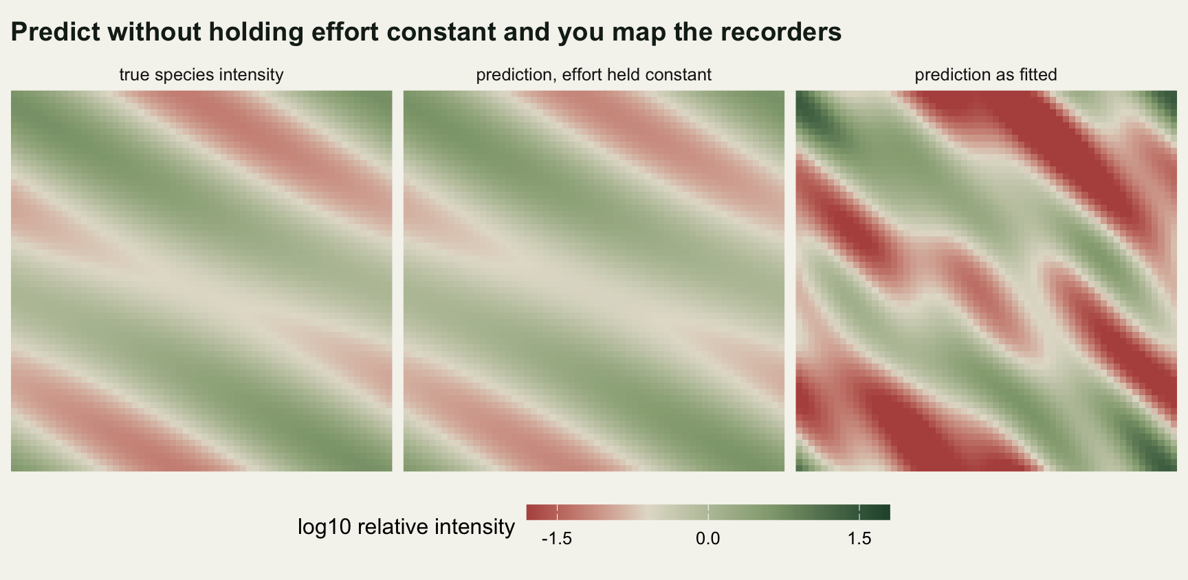

Figure 2: The true relative intensity, the prediction with effort held at a constant, and the prediction taken straight from the fitted model. All three come from the same fit.

All of that assumed the effort surface is known. It rarely is. What people have instead is a proxy: distance to road, distance to town, a kernel density of all records in the group. The sweep below degrades the proxy from a perfect copy of the effort surface down to something uncorrelated with it, keeping the noise component orthogonal to the environment so that the only thing changing is proxy quality.

set.seed(6161)
noise_f <- zstd(residuals(lm(smooth_field(gx, gy, 8, 5) ~ env + eff_ref)))
q_seq <- c(0, 0.3, 0.5, 0.7, 0.85, 0.95, 1)
n_rep_q <- 12
prox <- data.frame(quality = q_seq, slope = 0)
for (i in seq_along(q_seq)) {
  px <- zstd(q_seq[i] * eff_ref + sqrt(1 - q_seq[i]^2) * noise_f)
  cv <- data.frame(env = env, eff = px)
  prox$slope[i] <- mean(replicate(n_rep_q,
    coef(fit_pb(draw_records(eff_ref), uni_bg(), pres ~ env + eff, cv))[2]))
}
naive_ref <- sweep_rows$naive[sweep_rows$rho == 0.6]
prox$err_pct <- 100 * (prox$slope / b_env - 1)
prox$removed_pct <- 100 * (1 - (prox$slope - b_env) / (naive_ref - b_env))
print(round(prox, 2))

  quality slope err_pct removed_pct
1    0.00  1.85   53.82       -1.69
2    0.30  1.83   52.76        0.31
3    0.50  1.82   51.52        2.65
4    0.70  1.73   44.58       15.76
5    0.85  1.60   33.53       36.65
6    0.95  1.36   13.29       74.88
7    1.00  1.19   -0.96      101.82

The correction is worth much less than its correlation suggests. A proxy correlated 0.7 with the true effort surface removes 15.76 per cent of the bias and leaves the slope at 1.73. At 0.85 it removes 36.65 per cent. Only above 0.95, where the proxy removes 74.88 per cent, does the exercise start to pay. The reason is the usual attenuation of a mismeasured covariate: the coefficient on the proxy shrinks towards zero, so the effort term absorbs less of the pattern than it should, and the environment picks up the remainder. A weak proxy is not a partial solution in proportion to its quality; it is close to no solution at all.

Target-group background, and the assumption it rests on

The second remedy needs no effort layer. Draw the background points from records of other species collected the same way: the same recorders, the same traps, the same herbarium. If those records carry the same effort pattern as the focal species, the pattern appears in both the numerator and the denominator of the density ratio and cancels.

In the sweep table the tgb column runs from 1.188 to 1.202 across the whole correlation range: the same performance as the effort covariate, without needing an effort surface. The case against it is that the cancellation is exact only when the target group’s bias matches the focal species’ bias, and nobody checks. The sweep below varies the target group’s effort slope as a multiple of the focal species’ effort slope, from a group with no bias at all to a group with half again as much.

set.seed(7272)
kap_seq <- c(0, 0.25, 0.5, 0.75, 1, 1.25, 1.5)
n_rep_k <- 12
tgs <- data.frame(match = kap_seq, slope = 0)
for (i in seq_along(kap_seq)) {
  wt <- exp(kap_seq[i] * g_eff * eff_ref)
  tgs$slope[i] <- mean(replicate(n_rep_k, {
    tg <- sample(seq_len(n_cell), n_bg, replace = TRUE, prob = wt)
    coef(fit_pb(draw_records(eff_ref), tg, pres ~ env, covs_ref))[2] }))
}
tgs$err_pct <- 100 * (tgs$slope / b_env - 1)
print(round(tgs, 2))

  match slope err_pct
1  0.00  1.85   54.38
2  0.25  1.70   41.31
3  0.50  1.53   27.64
4  0.75  1.39   15.99
5  1.00  1.21    0.46
6  1.25  1.01  -15.79
7  1.50  0.86  -28.18

The relationship is close to a straight line through the truth at a match of 1. A target group with three quarters of the focal species’ bias leaves 15.99 per cent of error; a group with half of it leaves 27.64 per cent, which is barely better than doing nothing at the same correlation. Overshooting is symmetric and no safer: a group with one and a quarter times the bias gives -15.79 per cent, and the slope keeps falling from there. To stay inside a ten per cent error band the target group has to sit within roughly a sixth of the focal species’ bias in either direction.

That is demanding, and it is the assumption nobody states. A target group is usually chosen as everything in the same taxonomic group collected by the same method, which controls for who was out looking but not for what they were looking for. A group whose members are conspicuous, or seasonally obvious, or of interest to specialists, carries a different effort signature from a focal species that is none of those things.

p_tgb <- ggplot(tgs, aes(match, slope)) +
  geom_ribbon(aes(ymin = 0.9 * b_env, ymax = 1.1 * b_env), fill = te_pal$sage, alpha = 0.28) +
  geom_hline(yintercept = b_env, colour = te_pal$ink, linewidth = 0.7) +
  geom_hline(yintercept = naive_ref, colour = te_pal$clay, linetype = "22", linewidth = 0.7) +
  geom_line(colour = te_pal$green, linewidth = 0.9) +
  geom_point(colour = te_pal$forest, size = 2.6) +
  annotate("text", x = 0.02, y = b_env - 0.07, hjust = 0, size = 3.3,
           colour = te_pal$ink, label = "truth, with a 10 per cent band") +
  annotate("text", x = 1.48, y = naive_ref - 0.07, hjust = 1, size = 3.3,
           colour = te_pal$clay, label = "naive fit") +
  labs(title = "The target group has to share the bias",
       x = "target-group bias as a multiple of the focal species' bias",
       y = "recovered environmental slope") +
  theme_te()
print(p_tgb)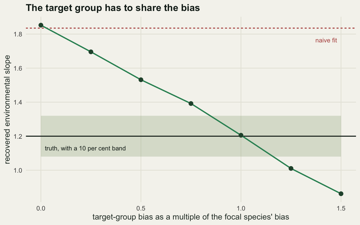

Figure 3: Recovered environmental slope against the degree to which the target group shares the focal species’ sampling bias. The band marks a ten per cent error around the truth.

Spatial thinning removes duplication, not effort bias

The third remedy is the cheapest to apply and the most popular: reduce the occurrences to at most one per grid cell, or to one per fixed radius, and fit as before. Two versions are measured below, at zero correlation and at 0.6, with the model-based standard error and the replicate-to-replicate spread of the estimate reported alongside the count of survivors.

thin_radius <- function(ii, jj, rad) {
  keep <- integer(0)
  for (k in sample(seq_along(ii))) {
    if (length(keep) == 0L) { keep <- k; next }
    if (min((ii[keep] - ii[k])^2 + (jj[keep] - jj[k])^2) >= rad^2) keep <- c(keep, k)
  }
  keep
}
rad_cells <- 3
n_rep_t <- 15
set.seed(8181)
thin_rows <- NULL
for (rh in c(0, 0.6)) {
  effv <- make_effort(rh); covs <- data.frame(env = env, eff = effv)
  acc <- matrix(0, n_rep_t, 9)
  for (r in seq_len(n_rep_t)) {
    rc <- draw_records(effv); bc <- uni_bg()
    kp <- thin_radius(gx[rc], gy[rc], rad_cells)
    ma <- fit_pb(rc, bc, pres ~ env, covs)
    mb <- fit_pb(unique(rc), bc, pres ~ env, covs)
    mc <- fit_pb(rc[kp], bc, pres ~ env, covs)
    acc[r, ] <- c(coef(ma)[2], coef(mb)[2], coef(mc)[2],
                  summary(ma)$coefficients[2, 2], summary(mb)$coefficients[2, 2],
                  summary(mc)$coefficients[2, 2], length(rc), length(unique(rc)), length(kp))
  }
  thin_rows <- rbind(thin_rows, data.frame(rho = rh,
    scheme = c("all records", "one per cell", "one per radius"),
    kept = round(colMeans(acc)[7:9]), slope = colMeans(acc)[1:3],
    err_pct = 100 * (colMeans(acc)[1:3] / b_env - 1),
    model_se = colMeans(acc)[4:6], spread = apply(acc[, 1:3], 2, sd)))
}
print(round(thin_rows[, -2], 3))

  rho kept slope err_pct model_se spread
1 0.0 1288 1.216   1.352    0.040  0.042
2 0.0  758 0.859 -28.390    0.045  0.041
3 0.0  163 0.425 -64.565    0.083  0.045
4 0.6 1365 1.837  53.064    0.052  0.064
5 0.6  698 1.278   6.530    0.055  0.041
6 0.6  142 0.692 -42.312    0.094  0.035

print(as.character(thin_rows$scheme))

[1] "all records"    "one per cell"   "one per radius" "all records"   
[5] "one per cell"   "one per radius"

cat(sprintf("thinning radius %d cells; replicate datasets %d\n", rad_cells, n_rep_t))

thinning radius 3 cells; replicate datasets 15

cat(sprintf("at zero correlation, error of one per cell %.1f per cent, one per radius %.1f\n",
            thin_rows$err_pct[2], thin_rows$err_pct[3]))

at zero correlation, error of one per cell -28.4 per cent, one per radius -64.6

The result is not the one the practice implies. At zero correlation, where the naive fit was already right, one record per cell takes the slope from 1.216 down to 0.859, 28.4 per cent below the truth, and thinning to one per radius takes it to 0.425, or 64.6 per cent below the truth: a large error introduced where there was none to fix. At a correlation of 0.6 the cell version does land near the truth, 1.278 against 1.2, but only because a downward bias of its own has partly cancelled an upward bias of the data. Two errors of opposite sign are not a correction; move the correlation and the cancellation moves with it.

The cost side is equally plain. One per cell keeps 758 of 1288 records at zero correlation and the model standard error rises from 0.040 to 0.045; one per radius keeps 163 and the standard error doubles to 0.083. The replicate-to-replicate spread barely moves, which is its own warning: the thinned estimators are stable around the wrong number.

Two measurements pin down what is happening. The first is what thinning does to the composition of the sample; the second is the same thinning applied to a sparser version of the same species, where duplicate records within a cell are almost absent.

set.seed(2424)
eff0 <- make_effort(0)
rc <- draw_records(eff0)
kp <- thin_radius(gx[rc], gy[rc], rad_cells)
cat(sprintf("mean environment: background %.3f, all records %.3f, one per cell %.3f, one per radius %.3f\n",
            mean(env), mean(env[rc]), mean(env[unique(rc)]), mean(env[rc[kp]])))

mean environment: background 0.000, all records 1.007, one per cell 0.756, one per radius 0.358

draw_sparse <- function(effv, scale_l) {
  det_p <- exp(g_eff * (effv - max(effv)))
  rep(seq_len(n_cell), rbinom(n_cell, rpois(n_cell, scale_l * lam0 * exp(b_env * env)), det_p))
}
covs0 <- data.frame(env = env, eff = eff0)
sat <- NULL
for (sl in c(1, 0.15)) {
  acc <- matrix(0, 12, 4)
  for (r in 1:12) {
    rr <- draw_sparse(eff0, sl); bc <- uni_bg()
    acc[r, ] <- c(coef(fit_pb(rr, bc, pres ~ env, covs0))[2],
                  coef(fit_pb(unique(rr), bc, pres ~ env, covs0))[2],
                  length(rr), length(unique(rr)))
  }
  sat <- rbind(sat, data.frame(intensity = sl, records = mean(acc[, 3]),
    occupied = mean(acc[, 4]), per_cell = mean(acc[, 3]) / mean(acc[, 4]),
    all_records = mean(acc[, 1]), one_per_cell = mean(acc[, 2])))
}
print(round(sat, 3))

  intensity  records occupied per_cell all_records one_per_cell
1      1.00 1299.667  746.833    1.740       1.241        0.863
2      0.15  191.417  168.083    1.139       1.273        1.148

The mean environment among the raw records is 1.007 against a background mean of zero, which is the signal the model is there to find. One record per cell drags it to 0.756 and one per radius to 0.358, nearer the background mean than the raw records. That is the mechanism: a cell with eight records and a cell with one become the same observation, so the intensity the model sees is squashed towards presence and absence, and the squashing is strongest exactly where the species is commonest.

The sparse run confirms it. At full intensity there are 1.74 records per occupied cell and thinning moves the slope from 1.241 to 0.863. At 15 per cent of that intensity there are 1.14 records per occupied cell and the same thinning moves it only from 1.273 to 1.148. Thinning costs what duplication gives it.

None of which makes thinning useless. It addresses spatial clustering from repeat visits to the same spot, which is a real problem for cross-validation and for any procedure that treats records as independent. It is simply not a treatment for effort bias, and on this simulation it is a net loss whenever the environmental slope is the quantity of interest.

Ranking the four

est_lv <- c("naive", "effort covariate", "target-group background", "one record per cell")
d_rank <- data.frame(rho = rep(sweep_rows$rho, 4),
  est = factor(rep(est_lv, each = nrow(sweep_rows)), levels = est_lv),
  slope = c(sweep_rows$naive, sweep_rows$effort, sweep_rows$tgb, sweep_rows$thinned))
p_rank <- ggplot(d_rank, aes(rho, slope, colour = est, shape = est)) +
  geom_hline(yintercept = b_env, colour = te_pal$ink, linewidth = 0.7) +
  geom_line(linewidth = 0.8) + geom_point(size = 2.8) +
  annotate("text", x = 0.8, y = b_env - 0.06, hjust = 1, size = 3.3,
           colour = te_pal$ink, label = "truth") +
  scale_colour_manual(values = c(te_pal$clay, te_pal$forest, te_pal$green, te_pal$gold)) +
  scale_shape_manual(values = c(16, 15, 17, 18)) +
  labs(title = "Only two of the four hold flat as the bias grows",
       x = "correlation between survey effort and environment",
       y = "recovered environmental slope", colour = NULL, shape = NULL) +
  theme_te() +
  theme(legend.position = "top")
print(p_rank)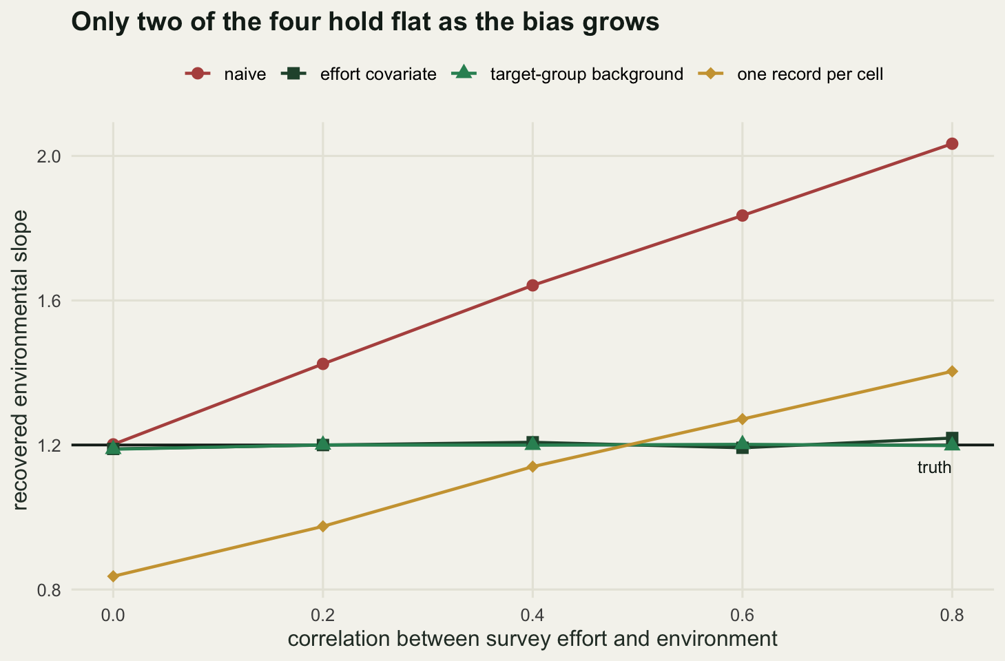

Figure 4: The four estimators across the effort-environment correlation grid, with the true environmental slope as a horizontal line. Each point averages 25 replicate datasets.

rank_tab <- data.frame(
  estimator = est_lv,
  mean_error = c(mean(abs(sweep_rows$naive - b_env)), mean(abs(sweep_rows$effort - b_env)),
                 mean(abs(sweep_rows$tgb - b_env)), mean(abs(sweep_rows$thinned - b_env))),
  worst_error = c(max(abs(sweep_rows$naive - b_env)), max(abs(sweep_rows$effort - b_env)),
                  max(abs(sweep_rows$tgb - b_env)), max(abs(sweep_rows$thinned - b_env))),
  spread = c(mean(sweep_rows$sd_naive), mean(sweep_rows$sd_effort),
             mean(sweep_rows$sd_tgb), mean(sweep_rows$sd_thin)))
rank_tab$needs <- c("nothing", "an effort surface", "a matched target group", "nothing")
rank_tab[, 2:4] <- round(rank_tab[, 2:4], 4)
print(rank_tab[order(rank_tab$mean_error), ], row.names = FALSE)

               estimator mean_error worst_error spread                  needs
 target-group background     0.0032      0.0117 0.0457 a matched target group
        effort covariate     0.0091      0.0193 0.0545      an effort surface
     one record per cell     0.1848      0.3634 0.0431                nothing
                   naive     0.4274      0.8339 0.0495                nothing

cat(sprintf("bias ranges over a factor of %.0f; replicate spread over a factor of %.2f\n",
            max(rank_tab$mean_error) / min(rank_tab$mean_error),
            max(rank_tab$spread) / min(rank_tab$spread)))

bias ranges over a factor of 134; replicate spread over a factor of 1.26

Ranked by mean absolute error over the correlation grid, target-group background comes first at 0.0032, the effort covariate second at 0.0091, one record per cell third at 0.1848 and the naive fit last at 0.4274. Ranked by replicate-to-replicate spread the ordering is nearly reversed and the differences are trivial: from 0.0431 for one record per cell to 0.0545 for the effort covariate, a factor of 1.26, against a factor of 134 in bias. Bias dominates, and by two orders of magnitude. There is no precision argument that rescues the naive fit.

Which to reach for depends on what you have, not on which scored better here. If a credible effort surface can be measured rather than guessed, the effort covariate is the one to use, because it also gives you the prediction step and a coefficient you can inspect. If the records came from a database holding comparable species collected the same way, target-group background is as good and asks for less. If the only side information is a weak proxy, be honest about what it buys: at a correlation of 0.7 with the truth it removes about a sixth of the bias. And if none of the three is available, a naive fit with a stated caveat beats a thinned fit with an unstated one.

What presence-only data cannot tell you

Every remedy above needs something the records themselves do not contain: a measured effort surface, a target group whose bias matches, or a proxy good enough to be worth including. Nothing in the point pattern supplies any of them, and the reason is not a shortage of cleverness.

set.seed(1313)
draw_preference <- function(effv) {
  rep(seq_len(n_cell), rpois(n_cell, 0.167 * lam0 * exp(b_env * env + g_eff * (effv - max(effv)))))
}
acc <- matrix(0, 15, 4)
for (r in 1:15) {
  ra <- draw_records(eff_ref); rb <- draw_preference(eff_ref); bc <- uni_bg()
  acc[r, ] <- c(coef(fit_pb(ra, bc, pres ~ env + eff, covs_ref))[2:3],
                coef(fit_pb(rb, bc, pres ~ env + eff, covs_ref))[2:3])
}
im <- colMeans(acc)
cat(sprintf("biased detection: environment %.3f, effort %.3f\n", im[1], im[2]))

biased detection: environment 1.200, effort 1.013

cat(sprintf("genuine preference: environment %.3f, effort %.3f\n", im[3], im[4]))

genuine preference: environment 1.175, effort 1.019

cat(sprintf("difference %.4f and %.4f, against a replicate spread of %.4f\n",
            im[1] - im[3], im[2] - im[4], sd(acc[, 1])))

difference 0.0246 and -0.0055, against a replicate spread of 0.0566

Two species are simulated here. The first is indifferent to accessibility and is recorded more often where access is easy. The second genuinely prefers accessible ground, by exactly the same log-linear amount, and is recorded perfectly wherever it occurs. The fitted coefficients are 1.200 and 1.013 for the first, 1.175 and 1.019 for the second: differences of 0.0246 and -0.0055 against a replicate spread of 0.0566. The two datasets are the same dataset as far as any estimator is concerned.

That is the honest limit, and it has a practical edge. Whether to hold effort constant when predicting depends on which of those two species you have, and the records cannot tell you: holding it constant is right for the first and wrong for the second, where accessibility is part of the habitat. The decision has to come from outside the data, from knowing that the covariate is a road layer rather than a soil layer, or from a survey designed so that effort is known rather than inferred. That is the argument for the integrated species distribution model, where a structured sample carries what the presence-only records cannot: not a better estimator, but the one extra dataset that makes the question answerable.

Where to go next

Nothing above checks whether the fitted model is any good, only whether its coefficient is right, and a model can have the right slope and still fit badly. The next tutorial, checking a presence-only model, covers residual diagnostics for point process fits, calibration against held-out records, and what a background sample can and cannot validate.

References

Phillips SJ, Dudik M, Elith J, Graham CH, Lehmann A, Leathwick J, Ferrier S 2009 Ecological Applications 19(1):181-197 (10.1890/07-2153.1)

Warton DI, Shepherd LC 2010 The Annals of Applied Statistics 4(3):1383-1402 (10.1214/10-AOAS331)

Merow C, Smith MJ, Silander JA 2013 Ecography 36(10):1058-1069 (10.1111/j.1600-0587.2013.07872.x)

Warton DI, Renner IW, Ramp D 2013 PLoS ONE 8(11):e79168 (10.1371/journal.pone.0079168)

Fithian W, Elith J, Hastie T, Keith DA 2015 Methods in Ecology and Evolution 6(4):424-438 (10.1111/2041-210X.12242)

Related tutorials

• MaxEnt as a Poisson point process
• Regularisation and features in MaxEnt
• Checking a presence-only model
• Pseudo-absence and background points