library(terra)
library(dplyr)
library(ggplot2)
library(tidyr)Pseudo-absence and background points for SDMs
R
terra
SDM
sampling
ecology tutorial
How many background points an SDM needs, why predicted values are relative rather than probabilities, and how case weights stabilise the scale, worked in R.
Updated 27 September 2026: a new section, Background drawn evenly in environmental space, measures what such a background does to the fitted optimum and to AUC, and the background section now carries a worked example.
A presence-only dataset has no zeros. To fit a binomial GLM, a logistic regression, or most other correlative models, you need something to contrast the presences against: a sample of the conditions available across the region, labelled absent. These points go by two names. Pseudo-absences are treated as if they were surveyed absences, usually few and sometimes placed away from known presences. Background points simply describe the available environment, usually many and drawn at random. The distinction matters less than three decisions that both share: how many points, where they come from, and how they are weighted. This post works through all three on the same synthetic landscape used to build the baseline SDM.
The landscape, niche and presences (identical to the baseline post)
pal_paper <- "#f5f4ee"; pal_ink <- "#16241d"; pal_body <- "#2c3a31"
pal_forest <- "#275139"; pal_label <- "#46604a"; pal_line <- "#dad9ca"; pal_faint <- "#5d6b61"
pal_gold <- "#c9b458"; pal_red <- "#b5534e"
theme_te <- function(base_size = 12) {
  theme_minimal(base_size = base_size) +
    theme(text = element_text(colour = pal_body),
          plot.title = element_text(colour = pal_ink, face = "bold", size = rel(1.05)),
          plot.subtitle = element_text(colour = pal_faint),
          axis.title = element_text(colour = pal_label), axis.text = element_text(colour = pal_body),
          panel.grid.minor = element_blank(),
          panel.grid.major = element_line(colour = pal_line, linewidth = 0.3),
          strip.text = element_text(colour = pal_ink, face = "bold"),
          legend.title = element_text(colour = pal_label),
          plot.background = element_rect(fill = pal_paper, colour = NA),
          panel.background = element_rect(fill = "#f5f4ee", colour = NA),
          legend.key = element_rect(fill = pal_paper, colour = NA), legend.position = "top")
}

set.seed(42)
r_template <- rast(nrows = 80, ncols = 80, xmin = 0, xmax = 80, ymin = 0, ymax = 80)
xy <- xyFromCell(r_template, 1:ncell(r_template))
temp_trend <- 22 - 0.18 * xy[, "y"]
temp_noise <- rast(r_template); values(temp_noise) <- rnorm(ncell(r_template), 0, 2)
temp_noise <- focal(temp_noise, w = 9, fun = mean, na.rm = TRUE)
temp <- rast(r_template); values(temp) <- temp_trend; temp <- temp + temp_noise; names(temp) <- "temp"
prec_trend <- 500 + 5 * xy[, "x"]
prec_noise <- rast(r_template); values(prec_noise) <- rnorm(ncell(r_template), 0, 60)
prec_noise <- focal(prec_noise, w = 9, fun = mean, na.rm = TRUE)
prec <- rast(r_template); values(prec) <- prec_trend; prec <- prec + prec_noise; names(prec) <- "prec"
env <- c(temp, prec)
temp_v <- values(temp)[, 1]; prec_v <- values(prec)[, 1]

suit_true <- exp(-((temp_v - 15)^2) / (2 * 2.2^2)) * exp(-((prec_v - 800)^2) / (2 * 110^2))
set.seed(101)
pres_cells <- sample(ncell(r_template), 300, prob = suit_true, replace = FALSE)
pres_df <- data.frame(pa = 1, temp = temp_v[pres_cells], prec = prec_v[pres_cells])
The species has 300 occurrence records, its optimum sits at 15 degrees and 800 mm, and the true niche is known only because the landscape is simulated. Everything below is a decision about the zero class.
How many background points
Background points sample the available environment, so too few of them describe it poorly and the fitted niche wanders. To see how much, draw background sets of increasing size, fit the GLM each time, and record the estimated temperature optimum (the peak of the response curve). Repeating the draw 40 times at each size shows the spread, not just one lucky fit.
opt_from_fit <- function(m, dat) {
  ts <- seq(min(dat$temp), max(dat$temp), length.out = 200)
  ps <- seq(min(dat$prec), max(dat$prec), length.out = 200)
  c(temp_opt = ts[which.max(predict(m, data.frame(temp = ts, prec = median(dat$prec)), type = "response"))],
    prec_opt = ps[which.max(predict(m, data.frame(temp = median(dat$temp), prec = ps), type = "response"))])
}
n_grid <- c(50, 100, 250, 500, 1000, 2500, 5000)
set.seed(303)
res1 <- do.call(rbind, lapply(n_grid, function(nb) {
  t(sapply(1:40, function(i) {
    bgc <- sample(ncell(r_template), nb)
    d <- rbind(pres_df, data.frame(pa = 0, temp = temp_v[bgc], prec = prec_v[bgc]))
    d <- d[complete.cases(d), ]
    m <- glm(pa ~ poly(temp, 2) + poly(prec, 2), data = d, family = binomial)
    c(n_bg = nb, opt_from_fit(m, d))
  }))
}))
res1 <- as.data.frame(res1)
res1 %>% group_by(n_bg) %>%
  summarise(temp_sd = round(sd(temp_opt), 3), temp_mean = round(mean(temp_opt), 2),
            prec_sd = round(sd(prec_opt), 1), .groups = "drop")
# A tibble: 7 × 4
n_bg temp_sd temp_mean prec_sd
<dbl> <dbl> <dbl> <dbl>
1 50 0.226 14.8 39.3
2 100 0.201 14.9 29.9
3 250 0.137 14.9 15
4 500 0.099 14.9 12.4
5 1000 0.061 14.9 8.5
6 2500 0.038 14.9 4
7 5000 0.034 14.9 1.7The mean estimate sits near 14.9 at every size, so more background points do not move the answer, they sharpen it. The scatter in the estimated temperature optimum falls from a standard deviation of 0.23 at 50 points to 0.03 at 5000; for precipitation it falls from 39 to under 2. Below a few hundred points the niche estimate is visibly noisy.
res1_f <- res1 %>% mutate(n_bg = factor(n_bg, levels = n_grid))
ggplot(res1_f, aes(n_bg, temp_opt)) +
  geom_hline(yintercept = 15, colour = pal_red, linetype = "dashed") +
  geom_jitter(width = 0.12, height = 0, colour = pal_forest, alpha = 0.4, size = 1) +
  stat_summary(fun = mean, geom = "point", colour = pal_ink, size = 2.4) +
  annotate("text", x = 6.7, y = 15, label = "true optimum", colour = pal_red, hjust = 1, vjust = -0.4, size = 3.3) +
  labs(title = "Estimated temperature optimum by number of background points",
       subtitle = "40 background draws per level; black points are the mean of each",
       x = "Number of background points", y = "Estimated optimum (C)") +
  theme_te(12) + theme(legend.position = "none")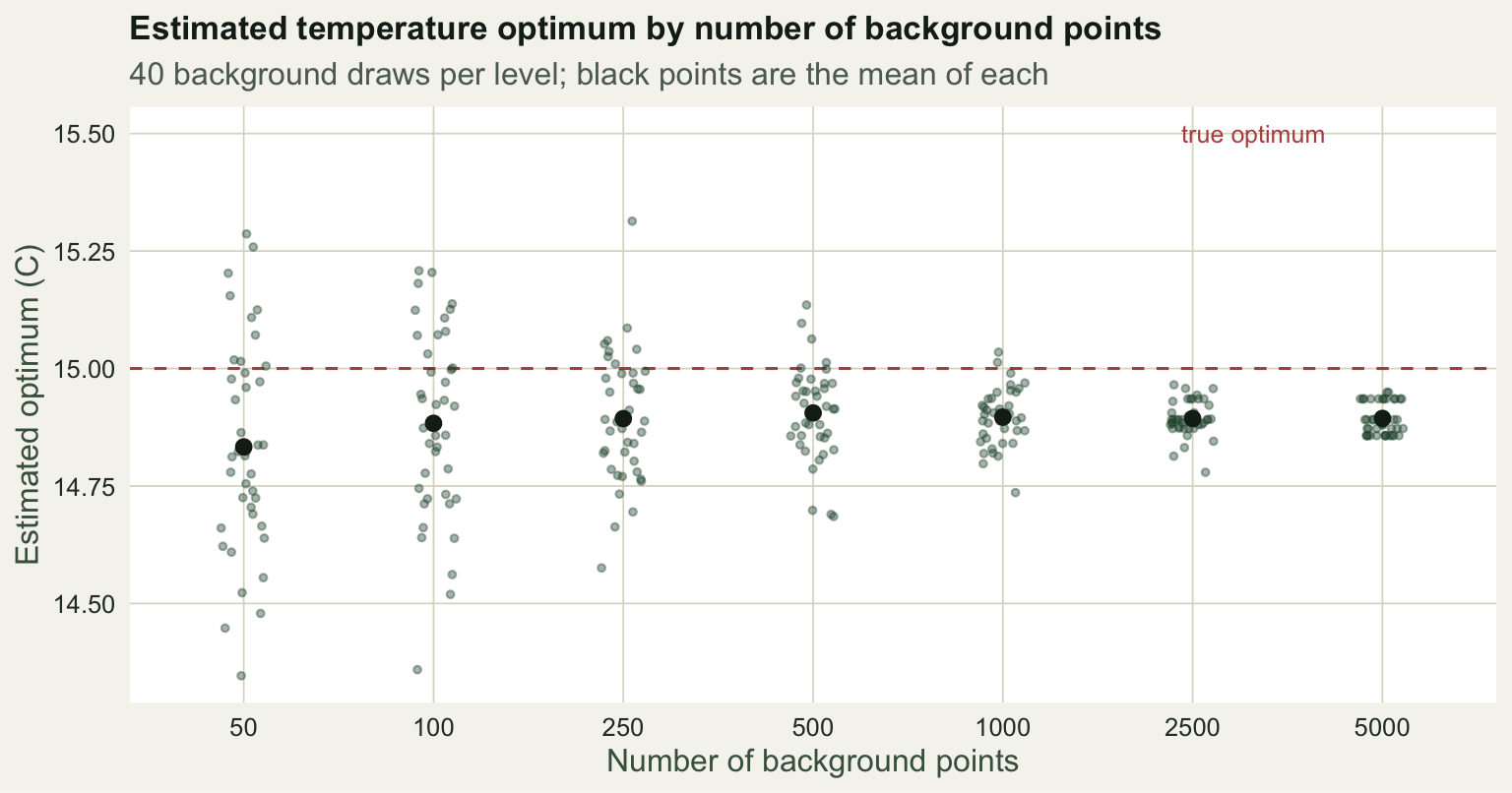
A common default is a large random background, in the thousands, precisely so this sampling noise stops mattering. The cost is only computation.
Predicted values are relative, not probabilities
There is a catch that more points cannot fix. The ratio of presences to background is something you choose, and that ratio sets the intercept of the logistic model. Change the number of background points and the predicted values shift up or down, even though the fitted shape does not move. Fit the same model with 500 and with 5000 background points and compare.
fit_glm <- function(nb, seed, weighted = FALSE) {
  set.seed(seed); bgc <- sample(ncell(r_template), nb)
  d <- rbind(pres_df, data.frame(pa = 0, temp = temp_v[bgc], prec = prec_v[bgc]))
  d <- d[complete.cases(d), ]
  w <- if (weighted) ifelse(d$pa == 1, 1, sum(d$pa == 1) / sum(d$pa == 0)) else rep(1, nrow(d))
  glm(pa ~ poly(temp, 2) + poly(prec, 2), data = d, family = binomial, weights = w)
}
m_500 <- fit_glm(500, 11); m_5000 <- fit_glm(5000, 11)
axis_t <- seq(min(temp_v), max(temp_v), length.out = 200)
curve_t <- function(m) predict(m, data.frame(temp = axis_t, prec = median(pres_df$prec)), type = "response")
c(intercept_500 = round(coef(m_500)[[1]], 2), intercept_5000 = round(coef(m_5000)[[1]], 2),
  peak_500 = round(max(curve_t(m_500)), 2), peak_5000 = round(max(curve_t(m_5000)), 2))
intercept_500 intercept_5000 peak_500 peak_5000
-0.93 -3.80 0.72 0.20 The intercept drops from -0.93 to -3.80 and the peak of the response curve falls from 0.72 to 0.20. The optimum is unchanged at 14.9 in both. The two surfaces rank cells almost identically:
v500  <- values(terra::predict(env, m_500,  type = "response", na.rm = TRUE))[, 1]
v5000 <- values(terra::predict(env, m_5000, type = "response", na.rm = TRUE))[, 1]
round(cor(v500, v5000, method = "spearman", use = "complete.obs"), 3)
[1] 1A Spearman correlation of 1.00 means the ranking of suitability across the landscape is the same; only the numbers on the scale differ. This is the single most misread property of a presence-background SDM: the output is a relative suitability index, not a probability of occurrence. Reporting a cell as “0.72 suitable” is meaningless without stating the background used to produce it.
The fix is to weight the classes. Down-weighting the background so its total weight equals the number of presences pins the effective prevalence, and the predicted scale no longer shifts with the number of background points you drew. It buys comparability, not a probability: the peak is still an index. The point-process route is a different construction (Warton and Shepherd 2010): there the background points carry large weights standing for the area each one represents, and only then do the fitted values estimate an intensity.
mw_500 <- fit_glm(500, 11, weighted = TRUE); mw_5000 <- fit_glm(5000, 11, weighted = TRUE)
c(weighted_peak_500 = round(max(curve_t(mw_500)), 2),
  weighted_peak_5000 = round(max(curve_t(mw_5000)), 2))
weighted_peak_500 weighted_peak_5000
0.81 0.81 With weights the peak lands at 0.81 for both sample sizes. The figure puts the two schemes side by side: unweighted, the curves separate by sample size; weighted, they coincide.
resp2 <- rbind(
  data.frame(temp = axis_t, y = curve_t(m_500),   n_bg = "500",  scheme = "Unweighted"),
  data.frame(temp = axis_t, y = curve_t(m_5000),  n_bg = "5000", scheme = "Unweighted"),
  data.frame(temp = axis_t, y = curve_t(mw_500),  n_bg = "500",  scheme = "Down-weighted background"),
  data.frame(temp = axis_t, y = curve_t(mw_5000), n_bg = "5000", scheme = "Down-weighted background"))
resp2$scheme <- factor(resp2$scheme, levels = c("Unweighted", "Down-weighted background"))
ggplot(resp2, aes(temp, y, colour = n_bg)) +
  geom_line(linewidth = 1) +
  facet_wrap(~scheme) +
  scale_colour_manual(values = c("500" = pal_gold, "5000" = pal_forest), name = "Background points") +
  labs(title = "Predicted values are relative, not probabilities",
       subtitle = "Same presences and same niche shape; only the vertical scale moves",
       x = "Temperature (C)", y = "Predicted value") +
  theme_te(12)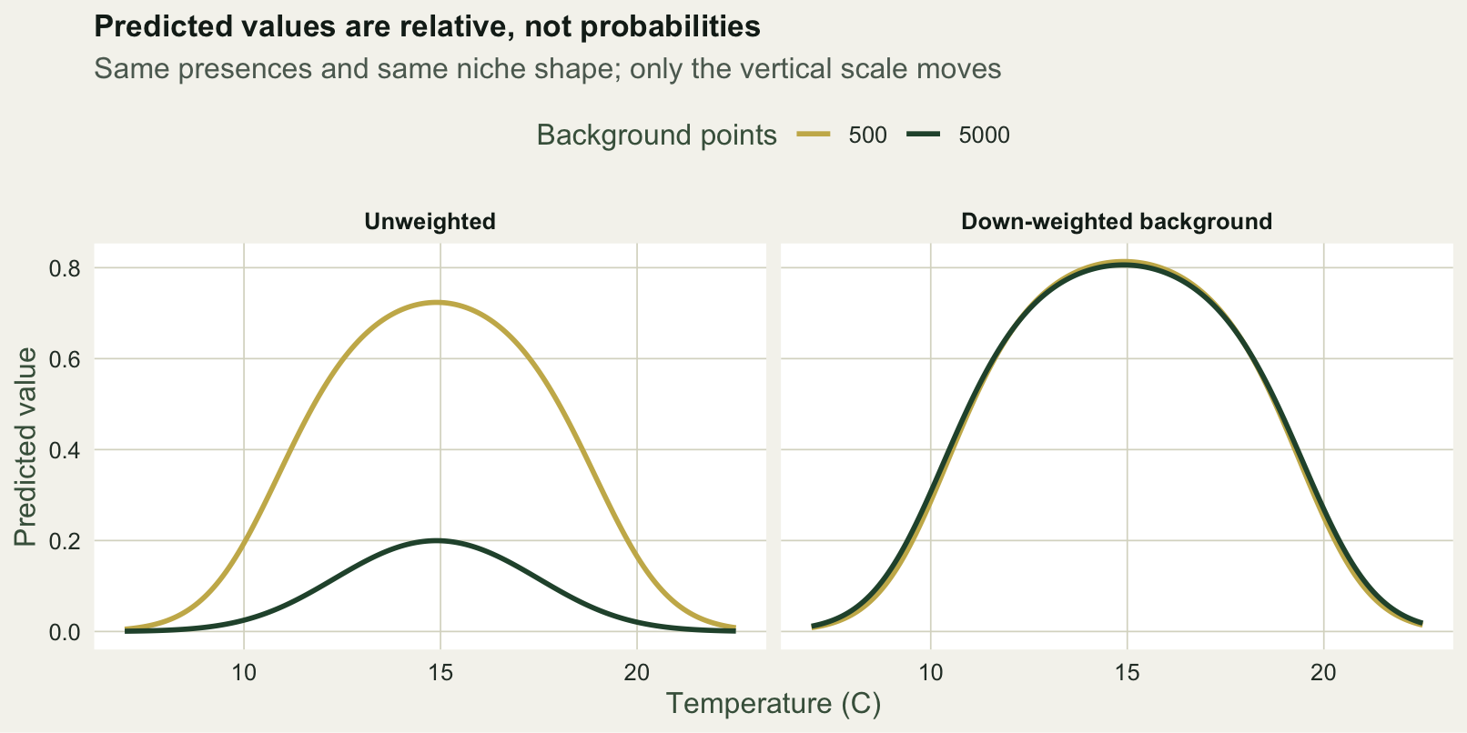
Where the background comes from
The third decision often matters most. Background drawn uniformly at random describes the whole region, which is the right reference only if occurrences were collected evenly across it. They rarely are. Records cluster near roads, towns and reserves, so the presences carry a sampling bias that random background does not share, and the model then partly fits survey effort rather than the species. One remedy is to draw background with the same bias as the occurrences, for example a target-group background built from records of similar, similarly surveyed species (Phillips et al. 2009).
Restricting the background to an accessible area, a buffer around the occurrences or a dispersal-limited region, changes the question the model answers. A wide background asks which conditions the species prefers across everything on offer; a narrow one asks how it sorts within the range it could plausibly reach. Neither is wrong, but they give different response curves, and the choice should follow the ecology, not the default (Barbet-Massin et al. 2012).
Background drawn evenly in environmental space
Some workflows spread the background evenly over environmental space instead of over the map: points uniform across the box of temperature and precipitation values the region spans, so that a rare climate gets as many points as a common one. A short argument says what that fit estimates. Presences arrive in proportion to a(x) lambda(x), where a(x) is how much of the region offers conditions x and lambda(x) is how strongly the species selects them. A background drawn at random across the map samples a(x), so the ratio the logistic model fits is lambda(x). A background flat in environmental space samples a constant, so the model fits a(x) lambda(x), and the response curve is centred on that product rather than on selection (a quadratic curve peaks near the product’s mean). This is the used-against-available logic of resource selection functions; availability sampling for step selection meets the same choice for step lengths.
On this landscape the two backgrounds should hardly differ, because both climate variables are gradients across a regular grid. Twenty draws of 5000 points each way, fitted with the same presences:
temp_bins <- table(cut(temp_v, 8)); prec_bins <- table(cut(prec_v, 8))
fit_opt <- function(bg) {
  d <- rbind(pres_df, data.frame(pa = 0, bg))
  opt_from_fit(glm(pa ~ poly(temp, 2) + poly(prec, 2), data = d, family = binomial), d)
}
set.seed(2027)
env_host <- t(replicate(20, {
  geo <- sample(ncell(r_template), 5000)
  bg_box <- data.frame(temp = runif(5000, min(temp_v), max(temp_v)), prec = runif(5000, min(prec_v), max(prec_v)))
  c(fit_opt(data.frame(temp = temp_v[geo], prec = prec_v[geo])), fit_opt(bg_box))
}))
colnames(env_host) <- c("temp_geo", "prec_geo", "temp_flat", "prec_flat")
temp_bins; prec_bins
(6.95,8.91] (8.91,10.9] (10.9,12.8] (12.8,14.7] (14.7,16.7] (16.7,18.6]
        609         829         862         904         888         816
(18.6,20.6] (20.6,22.5]
        817         675
(486,540] (540,593] (593,647] (647,701] (701,754] (754,808] (808,862] (862,916]
679 832 855 825 893 893 825 598 round(colMeans(env_host), 2) temp_geo prec_geo temp_flat prec_flat
14.89 791.16 14.84 769.90 Eight equal temperature bins hold between 609 and 904 cells, the emptiest at the two ends, and the temperature optimum is 14.89 with the geographic background against 14.84 with the flat one. Precipitation moves further, from 791 to 770 mm, or 0.19 of the niche’s 110 mm standard deviation against 0.02 for temperature, because the cells thin out at the wet end (the top bin holds 598 cells, the fullest 893), so a(x) lambda(x) is centred below the true 800 mm. Where availability is even, as it is for temperature, there is little for the flat background to change; the thin wet end already moves precipitation.
To see the effect in temperature, at a size set by design, the region has to offer some climates more than others. The next chunk builds such regions from this landscape: 3000 cells drawn with weight exp(s (temp - mean temp)), so that warm ground is scarce with s = -0.15 and common with s = 0.3. In each of 100 regions per slope, 300 presences come from the same true niche and the model is fitted twice, against 3000 geographic background points and against 3000 points uniform over the region’s temperature and precipitation ranges. AUC is scored on fresh presences against fresh geographic background, as an evaluation would do it; the Spearman correlation compares each prediction with the true suitability over the region’s cells.
fit_bg <- function(pres, bg) glm(pa ~ poly(temp, 2) + poly(prec, 2), family = binomial,
                                 data = rbind(pres, data.frame(pa = 0, bg)))
auc_rank <- function(s1, s0) (sum(rank(c(s1, s0))[seq_along(s1)]) - length(s1) * (length(s1) + 1) / 2) /
  (length(s1) * length(s0))
region_run <- function(slope) {
  reg <- sample(ncell(r_template), 3000, prob = exp(slope * (temp_v - mean(temp_v))))
  cells <- function(cc) data.frame(temp = temp_v[cc], prec = prec_v[cc])
  pres <- data.frame(pa = 1, cells(sample(reg, 300, prob = suit_true[reg])))
  bg_geo <- cells(sample(reg, 3000, replace = TRUE))
  bg_flat <- data.frame(temp = runif(3000, min(temp_v[reg]), max(temp_v[reg])),
                        prec = runif(3000, min(prec_v[reg]), max(prec_v[reg])))
  m_geo <- fit_bg(pres, bg_geo); m_flat <- fit_bg(pres, bg_flat)
  grid_d <- rbind(pres, data.frame(pa = 0, bg_geo))
  test_p <- cells(sample(reg, 300, prob = suit_true[reg])); test_b <- cells(sample(reg, 3000, replace = TRUE))
  c(opt_geo = opt_from_fit(m_geo, grid_d)[[1]], opt_flat = opt_from_fit(m_flat, grid_d)[[1]],
    pres_mean = mean(pres$temp),
    auc_geo = auc_rank(predict(m_geo, test_p), predict(m_geo, test_b)),
    auc_flat = auc_rank(predict(m_flat, test_p), predict(m_flat, test_b)),
    rho_geo = cor(predict(m_geo, cells(reg)), suit_true[reg], method = "spearman"),
    rho_flat = cor(predict(m_flat, cells(reg)), suit_true[reg], method = "spearman"))
}
set.seed(2028)
env_reg <- lapply(c(scarce = -0.15, common = 0.3), function(s) t(replicate(100, region_run(s))))
env_mean <- sapply(env_reg, colMeans)
env_mcse <- sapply(env_reg, function(r) apply(r, 2, sd) / sqrt(nrow(r)))
stopifnot(abs(env_mean["opt_geo", ] - 15) < 0.2)
round(env_mean, 3)
scarce common
opt_geo 14.978 15.013
opt_flat 14.404 15.940
pres_mean 14.386 15.937
auc_geo 0.810 0.806
auc_flat 0.803 0.789
rho_geo 0.997 0.996
rho_flat 0.973 0.948With warm ground scarce, the geographic background puts the temperature optimum at 14.98 and the flat background at 14.40; with warm ground common, at 15.01 and 15.94 (Monte Carlo standard errors at most 0.018 C). The flat fit moves towards the climate the region has most of, by 0.57 and 0.93 C, which is 0.26 and 0.42 of the niche’s standard deviation of 2.2 C. Its peak lands next to the mean temperature of the presences themselves (14.39 and 15.94), as the argument above predicts: the presences are a sample from a(x) lambda(x), and against a flat reference the quadratic takes the centre and spread of that sample. That centre is not the highest point of a(x) lambda(x) on this lumpy landscape, which moves with how finely the product is smoothed; a more flexible curve would follow the lumps.
Evaluation hardly registers the move. Held-out AUC is 0.810 against 0.803 in the first set of regions and 0.806 against 0.789 in the second, while the Spearman correlation with the true suitability falls from 0.997 to 0.973 and from 0.996 to 0.948. Neither background is wrong: the flat one estimates a(x) lambda(x), which answers where in this region the species is found, and the geographic one estimates lambda(x), which answers what it selects from what is on offer. The regions here are constructed, the model is the same quadratic GLM, and no sampling bias is simulated; the record bias described in the first paragraph of Where the background comes from (sampling bias in presence-only models) comes on top.
Recommendations
Use a large random background, in the low thousands, unless you have a specific reason not to; this removes the sampling noise from the first section. Treat the predictions as a relative index, and if you need a stable or comparable scale across models, weight the background as above. State plainly how many background points you used and where they came from, because as this post shows, both are part of the model rather than incidental settings. If the background was drawn evenly in environmental space, say so, because the fitted curve then describes where the species is found, not what it selects. The next step is measuring whether any of it predicts held-out occurrences, which is where evaluation comes in.
References
- Barbet-Massin M, Jiguet F, Albert CH, Thuiller W 2012. Methods in Ecology and Evolution 3(2):327-338 (10.1111/j.2041-210X.2011.00172.x)
- Phillips SJ, Dudik M, Elith J, Graham CH, Lehmann A, Leathwick J, Ferrier S 2009. Ecological Applications 19(1):181-197 (10.1890/07-2153.1)
- Warton DI, Shepherd LC 2010. The Annals of Applied Statistics 4(3):1383-1402 (10.1214/10-AOAS331)
- Guisan A, Zimmermann NE 2000. Ecological Modelling 135(2-3):147-186 (10.1016/S0304-3800(00)00354-9)