library(ggplot2)
te_canvas <- theme(plot.background  = element_rect(fill = "#f5f4ee", colour = NA),
                   panel.background = element_rect(fill = "#f5f4ee", colour = NA))
library(grid)

res_raw <- function(x, y) {
  1.5 * exp(-((x - 36)^2 + (y - 64)^2) / (2 * 22^2)) +
  1.2 * exp(-((x - 70)^2 + (y - 38)^2) / (2 * 24^2)) +
  (-0.00034) * ((x - 50)^2 + (y - 50)^2)
}
gx <- seq(0, 100, length.out = 120)
grid_df <- expand.grid(x = gx, y = gx)
grid_df$raw <- res_raw(grid_df$x, grid_df$y)
mu_r <- mean(grid_df$raw); sd_r <- sd(grid_df$raw)
resource <- function(x, y) (res_raw(x, y) - mu_r) / sd_r

rvm <- function(n, mu, kappa) {
  out <- numeric(n); a <- 1 + sqrt(1 + 4 * kappa^2)
  b <- (a - sqrt(2 * a)) / (2 * kappa); r <- (1 + b^2) / (2 * b)
  for (i in seq_len(n)) {
    repeat {
      u1 <- runif(1); u2 <- runif(1); u3 <- runif(1)
      z <- cos(pi * u1); f <- (1 + r * z) / (r + z); cc <- kappa * (r - f)
      if (cc * (2 - cc) - u2 > 0 || log(cc / u2) + 1 - cc >= 0) break
    }
    out[i] <- sign(u3 - 0.5) * acos(f) + mu
  }
  ((out + pi) %% (2 * pi)) - pi
}Availability sampling for step selection
movement ecology
habitat selection
R
ecology tutorial
How many available steps per used step, and from which distribution: extra steps buy precision in R, and the tentative kernel is a choice worth checking.
Every step selection analysis rests on a choice that is easy to make without thinking: how many available steps to pair with each used step, and what distribution to draw them from. This is the movement version of the question that haunts presence-background models, how many background points and from where. The two halves have different answers. The number of available steps controls how precisely you pin down the coefficients. The distribution they come from controls whether the coefficients are biased at all.
A track to sample against
We reuse the generative model from the earlier posts: an animal with a known movement kernel selecting for a resource with known strength. One track, so that everything downstream is a property of the sampling, not of a fresh simulation each time.
k_true <- 2.0; th_true <- 6.0; kap_true <- 0.9; beta_true <- 0.9
n <- 1500; M <- 300
set.seed(3141)
pos <- matrix(NA_real_, n + 1, 2); pos[1, ] <- c(46, 52)
heading <- numeric(n + 1); heading[1] <- runif(1, -pi, pi)
for (i in 1:n) {
  L <- rgamma(M, shape = k_true, scale = th_true); a <- rvm(M, 0, kap_true)
  ang <- heading[i] + a
  ex <- pos[i, 1] + L * cos(ang); ey <- pos[i, 2] + L * sin(ang)
  w <- exp(beta_true * resource(ex, ey)); j <- sample.int(M, 1, prob = w)
  pos[i + 1, ] <- c(ex[j], ey[j]); heading[i + 1] <- ang[j]
}
dx <- diff(pos[, 1]); dy <- diff(pos[, 2])
obs_l <- sqrt(dx^2 + dy^2); bearing <- atan2(dy, dx)
obs_turn <- ((diff(bearing) + pi) %% (2 * pi)) - pi
use_idx <- 2:n; n_str <- length(use_idx)

m1 <- mean(obs_l); v1 <- var(obs_l); k0 <- m1^2 / v1; th0 <- v1 / m1; lam0 <- 1 / th0
Cc <- mean(cos(obs_turn)); Ss <- mean(sin(obs_turn)); Rbar <- sqrt(Cc^2 + Ss^2); mu0 <- atan2(Ss, Cc)
kap0 <- if (Rbar < 0.53) 2 * Rbar + Rbar^3 + 5 * Rbar^5 / 6 else
        if (Rbar < 0.85) -0.4 + 1.39 * Rbar + 0.43 / (1 - Rbar) else
        1 / (Rbar^3 - 4 * Rbar^2 + 3 * Rbar)
How many available steps
A basic step selection function fits habitat as the only covariate, one used step against K available steps drawn from the tentative kernel. To separate the sampling noise from everything else, we fit the same track many times, redrawing the available steps each time, and watch how the estimate behaves as K grows.
fit_ssf <- function(Kk, sc, sh = k0, kp = kap0, seed) {
  set.seed(seed)
  Zc <- resource(pos[use_idx + 1, 1], pos[use_idx + 1, 2])
  Zm <- matrix(NA_real_, n_str, Kk)
  for (s in seq_along(use_idx)) {
    i <- use_idx[s]
    Ls <- rgamma(Kk, shape = sh, scale = sc); As <- rvm(Kk, mu0, kp)
    ang <- heading[i] + As
    Zm[s, ] <- resource(pos[i, 1] + Ls * cos(ang), pos[i, 2] + Ls * sin(ang))
  }
  Z <- cbind(Zc, Zm)
  o <- optim(0, function(b) { e <- Z * b; -sum(e[, 1] - log(rowSums(exp(e)))) },
             method = "BFGS", hessian = TRUE, control = list(reltol = 1e-9))
  c(est = o$par, se = sqrt(1 / o$hessian[1, 1]))
}

Kset <- c(1, 2, 5, 10, 20, 50, 100); R <- 40
setA <- data.frame()
for (Kk in Kset) {
  ests <- ses <- numeric(R)
  for (rr in 1:R) {
    fr <- fit_ssf(Kk, sc = th0, seed = 1000 * Kk + rr)
    ests[rr] <- fr["est"]; ses[rr] <- fr["se"]
  }
  setA <- rbind(setA, data.frame(K = Kk, mean_est = mean(ests),
                                 sd_est = sd(ests), mean_se = mean(ses)))
}
Two things move as K rises. The spread of the estimate across redraws, which is pure sampling noise from the availability set, falls from 0.053 at a single available step to 0.006 at a hundred. The model’s own standard error falls too, but it does not fall forever: it starts near 0.078 and settles around 0.053. That floor is set by the number of used steps, not by K. Once you have drawn enough available steps to integrate the availability well, adding more cannot tell you anything the 1499 observed steps do not already contain.
p_precision <- ggplot(setA, aes(K, mean_est)) +
  geom_hline(yintercept = beta_true, linetype = "dashed", colour = "#b5534e") +
  geom_ribbon(aes(ymin = mean_est - sd_est, ymax = mean_est + sd_est),
              fill = "#93a87f", alpha = 0.35) +
  geom_line(colour = "#275139", linewidth = 0.6) +
  geom_point(colour = "#275139", size = 2) +
  scale_x_log10(breaks = Kset) +
  annotate("text", x = 1.15, y = beta_true + 0.02, label = "true beta",
           colour = "#b5534e", size = 3, hjust = 0) +
  labs(x = "available steps per used step (K, log scale)",
       y = "habitat coefficient", title = "Habitat coefficient and redraw spread against K") +
  theme_minimal(base_size = 11) + te_canvas +
  theme(panel.grid.minor = element_blank(),
        plot.title = element_text(size = 10, colour = "#46604a"))
p_precision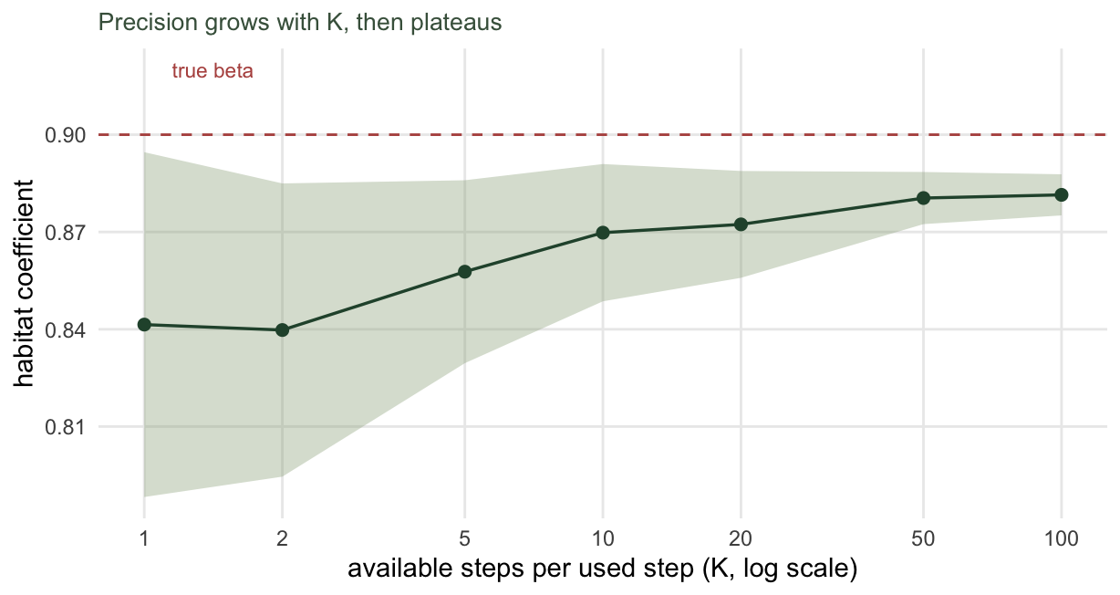
Notice where the curve settles: near the true value of 0.9, not on it. More available steps make the estimate tighter and steadier, but they do not close the remaining gap, and one simulated track fixes neither its size nor its sign. Part of that gap is bias from the contaminated tentative kernel, which no amount of sampling removes, and part is the single track you happen to be looking at. That is the second question.
What distribution to draw from
The available steps here come from a gamma fitted to the observed steps, which the earlier post showed is already shaped by selection. Does the choice matter? We take three tentative step-length distributions, one too short, one matched to the observed steps, one too long, and fit each with a basic step selection function and with the integrated version that carries movement covariates.
fit_issa <- function(sc, Kk = 15, seed = 77) {
  set.seed(seed)
  p <- 4; X <- matrix(NA_real_, n_str * (Kk + 1), p); row <- 1
  for (s in seq_along(use_idx)) {
    i <- use_idx[s]
    lu <- obs_l[i]; tu <- obs_turn[i - 1]
    X[row, ] <- c(resource(pos[i + 1, 1], pos[i + 1, 2]), log(lu), lu, cos(tu)); row <- row + 1
    Ls <- rgamma(Kk, shape = k0, scale = sc); As <- rvm(Kk, mu0, kap0)
    ang <- heading[i] + As
    ex <- pos[i, 1] + Ls * cos(ang); ey <- pos[i, 2] + Ls * sin(ang)
    X[row:(row + Kk - 1), ] <- cbind(resource(ex, ey), log(Ls), Ls, cos(As)); row <- row + Kk
  }
  nll <- function(b) { e <- as.vector(X %*% b); em <- matrix(e, nrow = Kk + 1)
                       -sum(em[1, ] - log(colSums(exp(em)))) }
  optim(rep(0, p), nll, method = "BFGS", control = list(reltol = 1e-9))$par[1]
}

scales <- c(0.6, 1.0, 1.6) * th0; labs <- c("too short", "matched", "too long")
setB <- data.frame()
for (m in seq_along(scales)) {
  b_basic <- fit_ssf(15, sc = scales[m], seed = 5000 + m)["est"]
  b_issa <- fit_issa(scales[m], Kk = 15, seed = 6000 + m)
  setB <- rbind(setB, data.frame(tentative = labs[m], basic = b_basic, issa = b_issa))
}
Here is what the choice does. The basic model’s habitat coefficient is 0.81 under the too-short kernel and 0.89 under the too-long one, and the integrated model returns 0.91, 0.95 and 0.95 across the same three kernels. Refit under more than one tentative kernel on your own track, and read how far each estimate travels before you trust either.
setB_long <- rbind(
  data.frame(tentative = setB$tentative, method = "basic SSF", est = setB$basic),
  data.frame(tentative = setB$tentative, method = "iSSA", est = setB$issa))
setB_long$tentative <- factor(setB_long$tentative, levels = labs)
ggplot(setB_long, aes(tentative, est, colour = method, group = method)) +
  geom_hline(yintercept = beta_true, linetype = "dashed", colour = "#b5534e") +
  geom_line(linewidth = 0.6) + geom_point(size = 2.8) +
  scale_colour_manual(values = c("basic SSF" = "#b5534e", "iSSA" = "#275139")) +
  annotate("text", x = 0.7, y = beta_true + 0.03, label = "true beta",
           colour = "#b5534e", size = 3, hjust = 0) +
  labs(x = "tentative step-length distribution", y = "habitat coefficient",
       colour = NULL, title = "Basic SSF and iSSA under three tentative kernels") +
  theme_minimal(base_size = 11) + te_canvas +
  theme(panel.grid.minor = element_blank(), legend.position = "inside", legend.position.inside = c(0.5, 0.14),
        legend.direction = "horizontal",
        legend.background = element_rect(fill = "#ffffff", colour = NA),
        plot.title = element_text(size = 10, colour = "#46604a"))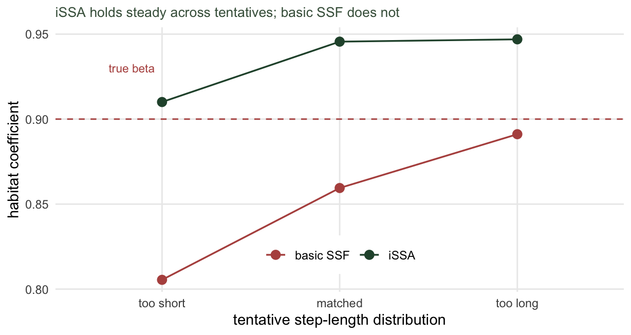
The integrated correction has limits of its own. It corrects the parametric form of the tentative kernel, so it needs available steps that actually cover the range the animal walked. A tentative so narrow that it never proposes a long step leaves the correction extrapolating into empty space, and eventually even the integrated estimate suffers. The three kernels here all overlap the observed steps.
What to do
For the number of available steps, do not stop at ten: the spread of the point estimate across redraws is still falling well past it. The standard error settles earlier, roughly flat from twenty upward, which is what makes it the wrong thing to watch. Raise the number of available steps until the estimate itself stops moving under redrawing, and past that you are spending computer time for nothing. For the distribution, fit the tentative kernel to the observed steps and refit under a shorter and a longer one, with and without movement covariates, so the dependence on that choice is something you measured rather than assumed. Whichever you pick, the fitted model still needs checking against the data it did not see, which is the final post in this thread.
References
Northrup JM, Hooten MB, Anderson CR, Wittemyer G 2013. Ecology 94(7):1456-1463 (10.1890/12-1688.1).
Forester JD, Im HK, Rathouz PJ 2009. Ecology 90(12):3554-3565 (10.1890/08-0874.1).
Avgar T, Potts JR, Lewis MA, Boyce MS 2016. Methods in Ecology and Evolution 7(5):619-630 (10.1111/2041-210X.12528).
Thurfjell H, Ciuti S, Boyce MS 2014. Movement Ecology 2:4 (10.1186/2051-3933-2-4).
Fortin D, Beyer HL, Boyce MS, Smith DW, Duchesne T, Mao JS 2005. Ecology 86(5):1320-1330 (10.1890/04-0953).
Fieberg J, Signer J, Smith B, Avgar T 2021. Journal of Animal Ecology 90(5):1027-1043 (10.1111/1365-2656.13441).