library(ggplot2)
library(patchwork)

te_paper  <- "#f5f4ee"
te_ink    <- "#16241d"
te_body   <- "#2c3a31"
te_forest <- "#275139"
te_rust   <- "#b5534e"
te_gold   <- "#c9b458"
te_line   <- "#dad9ca"

theme_datasheet <- function() {
  theme_minimal(base_size = 12) +
    theme(plot.background  = element_rect(fill = te_paper, colour = NA),
          panel.background = element_rect(fill = te_paper, colour = NA),
          panel.grid.major = element_line(colour = te_line, linewidth = 0.3),
          panel.grid.minor = element_blank(),
          text             = element_text(colour = te_body),
          plot.title       = element_text(colour = te_ink, face = "bold"),
          plot.subtitle    = element_text(colour = te_body),
          axis.text        = element_text(colour = te_body))
}SDM fitted before the invasion is over
R
SDM
invasion
species distributions
model checking
ecology tutorial
A presence-absence SDM fitted to a species still spreading puts its optimum at the founding site’s climate and maps a third of the potential range. In R.
An agency has ten years of standardised survey squares for a plant that arrived at a port, and a request for a map of where it could end up. The obvious thing to do is to fit a distribution model to the squares, since every square was visited and every square carries a presence or an absence, and then project the fitted response onto the whole country. The model fits well. The response curve is a clean unimodal function of temperature. The area under the curve on the survey data is high enough that nobody asks a second question.
The absences in those squares are of two kinds that the likelihood cannot tell apart. Some squares are empty because the plant cannot live there. Others are empty because the plant has not arrived yet, and those squares are not scattered at random: they lie beyond the front, which means they lie on one side of the climate gradient the plant is spreading along. The model reads “not reached” as “unsuitable” and the fitted niche comes out as a description of the invasion’s history.
Two posts on this site have already met that failure. Checking a metapopulation model fits an incidence function model to a network still climbing back from a crash and finds the area exponent near zero, with the reading that a near-zero exponent from a system you have reason to think is disturbed is a warning about equilibrium rather than a fact about patch size: the same transient read as biology, in another model’s costume. Checking a presence-only model states the species distribution case in prose and leaves it there, saying that a species still spreading occupies a subset of what suits it, so the fitted response describes the invasion front rather than the niche, and every diagnostic in that post will be satisfied. Neither gives the reader a number to compute for a distribution model fitted to a species that is still spreading.
This post supplies the numbers that sentence lacks, and the first of them is the reason for the check the post ends with: while the range is young, the fitted optimum sits on the climate of the founding site, so comparing the fitted optimum with the climate of the earliest records is a test of whether the model has learned anything the founders did not already say. The sections below build up to that check rather than opening with it, because two of the measurements are firmer than the check is. One is the curve: how wrong the fitted optimum and the predicted area are as a function of how full the range is, measured on a simulated invasion where the truth is known. The other is how much of a reported area is a property of the threshold rule rather than of the model. The check itself turns out to be one-sided, and it misses more of the cases it was built for than the size of the bias would suggest.
Two results here are known and are reproduced rather than discovered. Vaclavik and Meentemeyer fitted models to an invasion at several stages and found that early-stage models under-predict the potential distribution; Barve and colleagues set out the accessible area, the region a species could have reached, as the region a background or absence sample should come from. Elith, Kearney and Phillips set out the general problem of fitting a model to a species that is not in equilibrium with its climate, and what follows is one measurement inside that frame rather than an alternative to it. The accessible-area background is tested below as the obvious repair, using the buffer form that Pseudo-absence and background points for SDMs describes without running: restricting the background to an accessible area changes the question the model answers.
Most invader models are fitted to presence-only records, where a bias of this kind is easy to blame on the choice of background points. The case below is the harder one for that defence. Every square was visited, so every absence is a real absence, and the bias appears anyway.
A gradient, a niche and one introduction
The landscape is a square grid of cells. Temperature falls along one axis at a fixed rate and carries smoothed spatial noise on top, so the suitable band is a rough belt rather than a straight stripe. Suitability is a Gaussian function of temperature with an optimum of 16 degrees and a width of 3 degrees, and a cell counts as truly suitable when its suitability is above 0.3. That set is the denominator for every area figure below.
The species spreads as a stochastic contact process on the same grid. An empty cell is colonised with probability one minus the product over its occupied eight neighbours of one minus a per-neighbour rate proportional to suitability, and an occupied cell goes extinct with a probability that rises as suitability falls. Nothing about the process knows where the niche optimum is except through suitability, and no dispersal happens beyond the eight neighbours, so the range fills gradually from wherever it starts.
Everything in the two paragraphs above is a design constant, fixed before the simulation was run and not adjusted afterwards. The introduction point is the one deliberate contrast: three founding cells either at the warm margin of the niche, where suitability is between 0.35 and 0.5 and the temperature is above the optimum, which is the port-and-garden case, or in the middle of it, where suitability is above 0.9.
n_side     <- 40
t_opt_true <- 16
t_niche_sd <- 3
suit_cut   <- 0.3
col_rate   <- 0.35
ext_rate   <- 0.15
stage_gen  <- c(4, 8, 12, 16, 24, 40)
n_land     <- 40
buf_radius <- 5
n_found    <- 3

auc_stat <- function(score, lab) {
  rk <- rank(score)
  n1 <- sum(lab)
  n0 <- sum(!lab)
  (sum(rk[lab]) - n1 * (n1 + 1) / 2) / (n1 * n0)
}

smooth_field <- function(n, amp, r = 3) {
  z   <- matrix(rnorm((n + 2 * r)^2), n + 2 * r)
  out <- matrix(0, n, n)
  for (a in -r:r) for (b in -r:r)
    out <- out + exp(-(a^2 + b^2) / (2 * (r / 2)^2)) *
      z[(1 + r + a):(n + r + a), (1 + r + b):(n + r + b)]
  out / sd(out) * amp
}

neighbours8 <- function(M) {
  P <- matrix(0, n_side + 2, n_side + 2)
  P[2:(n_side + 1), 2:(n_side + 1)] <- M
  out <- matrix(0, n_side, n_side)
  for (a in -1:1) for (b in -1:1) if (a != 0 || b != 0)
    out <- out + P[(2 + a):(n_side + 1 + a), (2 + b):(n_side + 1 + b)]
  out
}

in_buffer <- function(M) {
  w <- buf_radius
  P <- matrix(0, n_side + 2 * w, n_side + 2 * w)
  P[(w + 1):(n_side + w), (w + 1):(n_side + w)] <- M
  out <- matrix(0, n_side, n_side)
  for (a in -w:w) for (b in -w:w)
    out <- out + P[(w + 1 + a):(n_side + w + a), (w + 1 + b):(n_side + w + b)]
  out > 0
}
The model fitted at each stage is a logistic regression of presence on temperature and its square, on every cell of the grid: the smallest model that can express a unimodal climatic response, and the one a practitioner writes first. Its optimum is minus the linear coefficient over twice the quadratic one.
Turning a fitted probability surface into a predicted area needs a threshold, and the choice matters more than it looks. The rule used here is the tenth percentile of the fitted values at the presence cells, which is standard practice and uses nothing but the training presences. Pearson and colleagues set out the lowest presence threshold, the lowest fitted value at any training record; the tenth-percentile variant used here drops the most marginal tenth of the records before taking that minimum, and how far apart the two rules are depends on how many presences there are. A second rule is carried through for comparison: cells whose fitted value is above 0.3 of the surface maximum, which is the rule that looks like the definition of the true suitable set but is applied to a quantity that is not suitability.
fit_sdm <- function(cells, keep) {
  ## fitted probabilities of 0 or 1 are expected on a sharp gradient and are
  ## harmless here, because only the two quadratic coefficients are used
  suppressWarnings(glm(pres ~ temp + I(temp^2), family = binomial,
                       data = cells[keep, ]))
}

optimum_of <- function(fit) {
  b <- coef(fit)
  if (b[3] < 0) -b[2] / (2 * b[3]) else NA_real_
}

area_pct10 <- function(pred, cells) {
  cut10 <- quantile(pred[cells$pres == 1], 0.10)
  sum(pred >= cut10) / sum(cells$truly)
}

area_rel <- function(pred, cells) {
  sum(pred / max(pred) > suit_cut) / sum(cells$truly)
}

## reads the fitted quadratic itself as a Gaussian suitability: the exponent of
## the linear predictor, recentred on its own peak, put through the same cut-off
area_gauss <- function(fit, cells) {
  b <- coef(fit)
  if (b[3] >= 0) return(NA_real_)
  shape <- exp(b[3] * (cells$temp + b[2] / (2 * b[3]))^2)
  sum(shape > suit_cut) / sum(cells$truly)
}
t_grid <- seq(8, 24, by = 0.25)
run_landscape <- function(placement, keep_maps = FALSE) {
row_id <- matrix(rep(seq_len(n_side), n_side), n_side, n_side)
temp <- 24 - 0.35 * (row_id - 1) + smooth_field(n_side, 1.2)
suit <- exp(-(temp - t_opt_true)^2 / (2 * t_niche_sd^2))
cells <- data.frame(temp = as.vector(temp), suit = as.vector(suit),
truly = as.vector(suit > suit_cut))
n_truly <- sum(cells$truly)
warm_unsuit <- sum(!cells$truly & cells$temp > t_opt_true)
cool_unsuit <- sum(!cells$truly & cells$temp <= t_opt_true)
pool <- if (placement == "warm margin") {
which(suit > 0.35 & suit < 0.5 & temp > t_opt_true)
} else {
which(suit > 0.9)
}
## founders come from the middle columns; on the occasional noise field that
## window holds fewer than n_found qualifying cells, so it widens until it
## does rather than the landscape being thrown away
win <- 2
while (sum(abs(((pool - 1) %/% n_side) + 1 - 20) <= win) < n_found) win <- win + 1
pool <- pool[abs(((pool - 1) %/% n_side) + 1 - 20) <= win]
occ <- matrix(0L, n_side, n_side)
founders <- sample(pool, n_found)
occ[founders] <- 1L
temp_found <- mean(temp[founders])
stats_out <- NULL
curve_out <- NULL
maps_out <- list()
for (g in seq_len(max(stage_gen))) {
p_col <- 1 - (1 - col_rate * suit)^neighbours8(occ)
nxt <- occ
nxt[occ == 0L & runif(n_side^2) < p_col] <- 1L
nxt[occ == 1L & runif(n_side^2) < ext_rate * (1 - suit)] <- 0L
occ <- nxt
if (g %in% stage_gen) {
cells$pres <- as.vector(occ)
all_fit <- fit_sdm(cells, rep(TRUE, nrow(cells)))
pred_all <- as.vector(predict(all_fit, newdata = cells, type = "response"))
buf_keep <- as.vector(in_buffer(occ))
buf_fit <- fit_sdm(cells, buf_keep)
pred_buf <- as.vector(predict(buf_fit, newdata = cells, type = "response"))
stats_out <- rbind(stats_out, data.frame(
placement = placement, gen = g,
fill = sum(cells$pres == 1 & cells$truly) / sum(cells$truly),
temp_found = temp_found,
temp_occ = mean(cells$temp[cells$pres == 1]),
opt = optimum_of(all_fit),
opt_buf = optimum_of(buf_fit),
area = area_pct10(pred_all, cells),
area_buf = area_pct10(pred_buf, cells),
area_r = area_rel(pred_all, cells),
area_r_buf = area_rel(pred_buf, cells),
auc_own = auc_stat(pred_all, cells$pres == 1),
auc_true = auc_stat(pred_all, cells$truly),
auc_tr_buf = auc_stat(pred_buf, cells$truly),
buf_share = mean(buf_keep),
area_g = area_gauss(all_fit, cells),
n_pres = sum(cells$pres),
sink_share = mean(!cells$truly[cells$pres == 1]),
n_truly = n_truly,
warm_un = warm_unsuit,
cool_un = cool_unsuit))
curve_p <- predict(all_fit, newdata = data.frame(temp = t_grid),
type = "response")
curve_out <- rbind(curve_out, data.frame(
placement = placement, gen = g, temp = t_grid,
shape = curve_p / max(curve_p)))
if (keep_maps) {
maps_out[[as.character(g)]] <- data.frame(
x = as.vector(col(occ)), y = as.vector(row(occ)),
temp = cells$temp, truly = cells$truly, pres = cells$pres == 1, gen = g)
}
}
}
list(stats = stats_out, curves = curve_out, maps = maps_out,
temp_found = temp_found)
}
set.seed(20260923)
sweep_out <- lapply(c("warm margin", "niche centre"), function(pl) {
lapply(seq_len(n_land), function(i) {
z <- run_landscape(pl, keep_maps = (i == 1L))
z$stats$land <- i
z$curves$land <- i
z
})
})
runs <- do.call(rbind, lapply(unlist(sweep_out, recursive = FALSE), `[[`, "stats"))
curves <- do.call(rbind, lapply(unlist(sweep_out, recursive = FALSE), `[[`, "curves"))
maps_1 <- sweep_out[[1]][[1]]$mapsmean_by <- function(v) {
ag <- aggregate(runs[[v]], list(placement = runs$placement, gen = runs$gen), mean)
names(ag)[3] <- v
ag
}
agg <- Reduce(function(a, b) merge(a, b, by = c("placement", "gen")),
lapply(c("fill", "temp_found", "temp_occ", "opt", "opt_buf",
"area", "area_buf", "area_r", "area_r_buf",
"auc_own", "auc_true", "auc_tr_buf", "buf_share",
"area_g", "n_pres", "sink_share"), mean_by))
agg$opt_err <- abs(agg$opt - t_opt_true)
agg$found_gap <- abs(agg$opt - agg$temp_found)
mar <- agg[agg$placement == "warm margin", ]
mar <- mar[order(mar$gen), ]
cen <- agg[agg$placement == "niche centre", ]
cen <- cen[order(cen$gen), ]
se_of <- function(v, pl, g) {
sd(runs[[v]][runs$placement == pl & runs$gen == g]) / sqrt(n_land)
}
se_opt_early <- se_of("opt", "warm margin", stage_gen[1])
se_area_early <- se_of("area", "warm margin", stage_gen[1])
n_stage <- length(stage_gen)
n_fit_total <- nrow(runs)
n_na_opt <- sum(is.na(runs$opt))
## landscape composition, and how many presences the threshold rule is given
truly_share <- mean(runs$n_truly) / n_side^2
warm_cool_rt <- mean(runs$warm_un) / mean(runs$cool_un)
n_pres_early <- runs$n_pres[runs$placement == "warm margin" &
runs$gen == stage_gen[1]]At the earliest stage the invasion has reached 2.6 per cent of the truly suitable cells for the warm-margin introduction, and at the last stage 93.3 per cent. Every number below is a mean over 40 independent landscapes, each with its own noise field and its own founding cells; the standard error of the mean fitted optimum at the earliest stage is 0.09 degrees and that of the mean area ratio is 0.017. All 480 fits produced a downward-curving quadratic, so a fitted optimum exists in every one of them (0 failures). The truly suitable set that every area ratio is divided by covers 65 per cent of the grid on average, and the unsuitable remainder holds about 2.8 warm cells for every cool one; both numbers matter for the rankings below.
map_early <- maps_1[[as.character(stage_gen[1])]]
map_late  <- maps_1[[as.character(stage_gen[n_stage])]]

base_map <- function(dat, ttl, show_occ) {
  g <- ggplot(dat, aes(x, y)) +
    geom_raster(aes(fill = temp)) +
    geom_contour(aes(z = as.numeric(truly)), breaks = 0.5,
                 colour = te_ink, linetype = "dashed", linewidth = 0.4)
  if (show_occ) {
    g <- g + geom_tile(data = dat[dat$pres, ], fill = te_rust, colour = NA)
  }
  g +
    scale_fill_gradient(low = te_paper, high = te_body, name = NULL) +
    coord_equal(expand = FALSE) +
    labs(x = NULL, y = NULL, subtitle = ttl) +
    theme_datasheet() +
    theme(axis.text = element_blank(), panel.grid = element_blank(),
          plot.subtitle = element_text(size = 10),
          legend.position = "none")
}

(base_map(map_early, "temperature", FALSE) +
   base_map(map_early, sprintf("occupied, generation %d", stage_gen[1]), TRUE) +
   base_map(map_late, sprintf("occupied, generation %d", stage_gen[n_stage]), TRUE)) +
  plot_annotation(
    title = "A warm-margin introduction filling a suitable band",
    subtitle = "dark: warm; dashed: the truly suitable set; red: occupied cells",
    theme = theme_datasheet())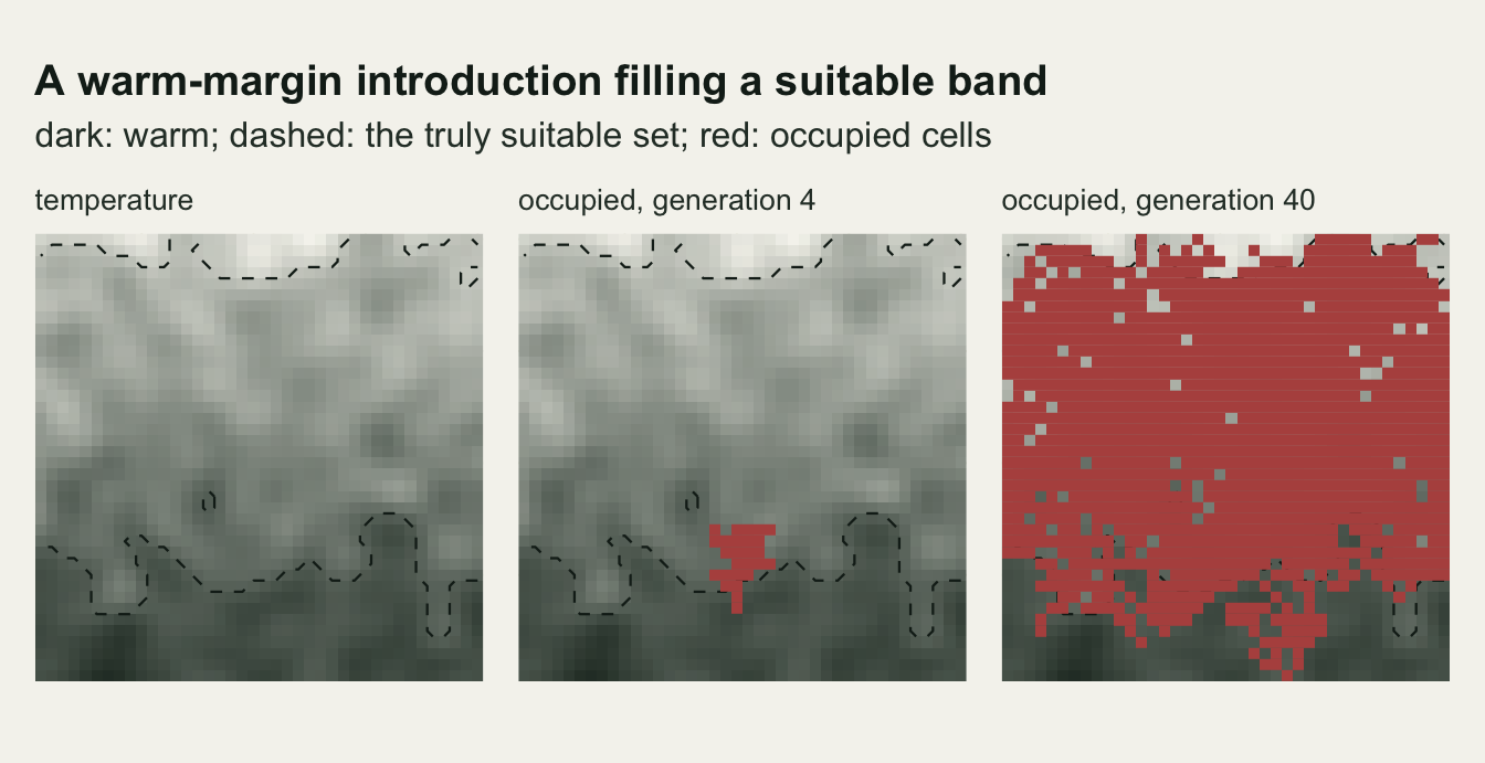
What the model says at each stage
The response curve the model reports is a clean unimodal function of temperature at every stage. What changes is where its peak sits. Below, each fitted curve is rescaled to its own maximum so that the shapes can be compared on one panel; the rescaling is cosmetic and none of the numbers in the text depend on it.
curve_mean <- aggregate(shape ~ placement + gen + temp, data = curves, FUN = mean)
curve_mean$stage <- factor(sprintf("gen %d", curve_mean$gen),
                           levels = sprintf("gen %d", stage_gen))
truth_df <- data.frame(temp = t_grid,
                       shape = exp(-(t_grid - t_opt_true)^2 / (2 * t_niche_sd^2)))
found_df <- data.frame(placement = c("warm margin", "niche centre"),
                       temp_found = c(mar$temp_found[1], cen$temp_found[1]))
stage_cols <- c(te_rust, "#c87f52", te_gold, "#8a9a54", te_forest, te_ink)

ggplot(curve_mean, aes(temp, shape, colour = stage)) +
  geom_line(data = truth_df, aes(temp, shape), inherit.aes = FALSE,
            colour = te_line, linewidth = 2) +
  geom_vline(data = found_df, aes(xintercept = temp_found),
             colour = te_rust, linetype = "dotted", linewidth = 0.6) +
  geom_line(linewidth = 0.8) +
  scale_colour_manual(values = stage_cols, name = NULL) +
  facet_wrap(~ placement) +
  labs(x = "temperature (degrees)", y = "response, rescaled to its own maximum",
       title = "The fitted peak starts at the founding climate",
       subtitle = "thick grey: true suitability; dotted red: mean founding temperature") +
  theme_datasheet() +
  theme(legend.position = "bottom", strip.text = element_text(colour = te_ink))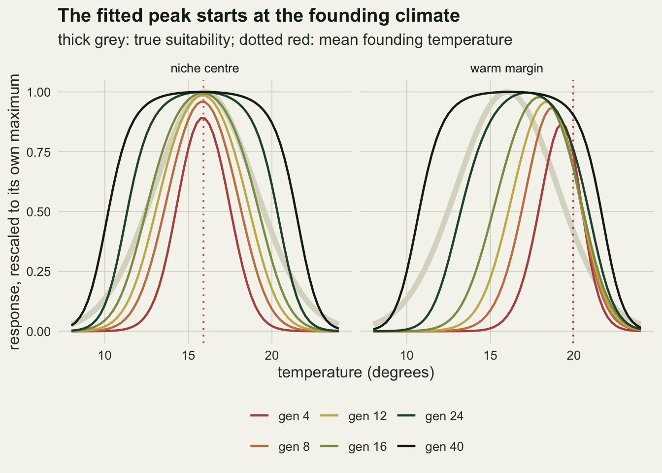
opt_first  <- mar$opt[1]
opt_last   <- mar$opt[n_stage]
found_mar  <- mar$temp_found[1]
gap_first  <- abs(opt_first - found_mar)
gap_last   <- abs(opt_last - found_mar)
occ_gap1   <- abs(opt_first - mar$temp_occ[1])
occ_gap_mx <- max(abs(mar$opt - mar$temp_occ))
mar_rows   <- runs[runs$placement == "warm margin", ]
occ_gap_wo <- max(abs(mar_rows$opt - mar_rows$temp_occ))
cen_opt_rng <- range(cen$opt)
cen_rows    <- runs[runs$placement == "niche centre", ]
cen_opt_sc  <- range(cen_rows$opt)
cen_worst   <- max(abs(cen_rows$opt - t_opt_true))
cen_found   <- cen$temp_found[1]
auc_own_rng <- range(mar$auc_own)
opt_seq_pre   <- abs(mar$opt - t_opt_true)
auc_own_worst <- mar$auc_own[which.max(abs(mar$opt - t_opt_true))]
auc_own_best  <- mar$auc_own[which.min(abs(mar$opt - t_opt_true))]
se_auc_own    <- sapply(stage_gen, function(g) se_of("auc_own", "warm margin", g))
auc_own_lo    <- min(mar$auc_own)
auc_own_hi    <- max(mar$auc_own)
se_auc_own_lo <- se_auc_own[which.min(mar$auc_own)]
se_auc_own_hi <- se_auc_own[which.max(mar$auc_own)]
For the warm-margin introduction the mean founding temperature is 19.9 degrees and the fitted optimum at the earliest stage is 19.2 degrees, 0.75 degrees away from it and 3.2 degrees away from the true optimum of 16. By the last stage the fitted optimum has moved to 16.2, which is 3.8 degrees from the founding climate. Nothing about the species changed between those two fits.
The optimum does not lag behind the occupied cells; it sits on them. The gap between the fitted optimum and the mean temperature of the currently occupied cells is 0.03 degrees at the earliest stage, and the stage mean of that gap never exceeds 0.16 degrees at any of the 6 stages of the warm-margin set, with the worst single landscape at 0.63 degrees. That is the mechanism in one line: the quadratic reports the centre of the occupied cloud, and early in an invasion the occupied cloud is the founding site.
The niche-centre introduction is the control that shows the founding site, not the invasion, is doing the work. There the founding cells average 15.9 degrees, close to the true optimum by construction, and the mean fitted optimum stays between 15.82 and 15.89 degrees at every stage. That is a statement about the bias and not about any one fit: single landscapes run from 14.1 to 17.6 degrees, and the worst control fit is 1.9 degrees out, which is more than half the earliest-stage warm-margin bias it is the control for. A practitioner reading only the response curve would call the average control model correct, and on average it is.
Meanwhile the internal check says nothing is wrong. Area under the curve on the model’s own presence-absence data, for the warm-margin set, ranges from 0.84 to 0.93 across the six stages. It is 0.88 at the stage where the optimum is furthest from the truth and 0.93 at the stage where it is closest, a difference of 0.05 between a fit whose optimum is 3.2 degrees out and one whose optimum is 0.2 degrees out, and it is lower in the middle than at either end. The move from 0.839 to 0.930 is many times its own standard error (0.005 and 0.002 respectively), so it is a real change; it is also a change nobody would act on, both ends being reported as a good fit, while the quantity of interest moves by everything. Fitting the data well and describing the niche are different achievements, and the first cannot be used as evidence of the second.
Two errors that decay as the range fills
The two quantities a manager actually uses are the optimum, which decides which regions get watched, and the predicted area, which decides how big the problem is. Both are wrong in the same direction early on, and both recover as the range fills.
dec <- rbind(
  data.frame(placement = agg$placement, fill = agg$fill,
             value = abs(agg$opt - t_opt_true), panel = "optimum error (degrees)",
             series = "fitted optimum"),
  data.frame(placement = agg$placement, fill = agg$fill,
             value = agg$area, panel = "predicted area / true area",
             series = "all cells"),
  data.frame(placement = agg$placement, fill = agg$fill,
             value = agg$auc_own, panel = "AUC", series = "on its own data"),
  data.frame(placement = agg$placement, fill = agg$fill,
             value = agg$auc_true, panel = "AUC", series = "against the truth"))
dec$panel <- factor(dec$panel, levels = c("optimum error (degrees)",
                                          "predicted area / true area", "AUC"))
hlines <- data.frame(panel = factor(c("predicted area / true area", "AUC"),
                                    levels = levels(dec$panel)),
                     yint = c(1, 0.5))
## the single landscapes behind the three solid series, so the spread is visible
dec_pts <- rbind(
  data.frame(placement = runs$placement, fill = runs$fill,
             value = abs(runs$opt - t_opt_true),
             panel = "optimum error (degrees)"),
  data.frame(placement = runs$placement, fill = runs$fill,
             value = runs$area, panel = "predicted area / true area"),
  data.frame(placement = runs$placement, fill = runs$fill,
             value = runs$auc_true, panel = "AUC"))
dec_pts$panel <- factor(dec_pts$panel, levels = levels(dec$panel))

ggplot(dec, aes(fill, value, colour = placement, linetype = series)) +
  geom_hline(data = hlines, aes(yintercept = yint),
             linetype = "dashed", colour = te_line, linewidth = 0.6) +
  geom_point(data = dec_pts, aes(fill, value, colour = placement),
             inherit.aes = FALSE, alpha = 0.16, size = 0.7) +
  geom_line(linewidth = 0.8) +
  geom_point(size = 1.8) +
  facet_wrap(~ panel, scales = "free_y") +
  scale_colour_manual(values = c("warm margin" = te_rust,
                                 "niche centre" = te_forest), name = NULL) +
  scale_linetype_manual(values = c("fitted optimum" = "solid",
                                   "all cells" = "solid",
                                   "on its own data" = "dotted",
                                   "against the truth" = "solid"),
                        guide = "none") +
  labs(x = "occupied share of the truly suitable cells",
       y = NULL, title = "Both errors decay as the range fills",
       subtitle = sprintf(paste("lines: means of %d landscapes; faint points:",
                                "single landscapes; dotted: AUC on own data"),
                          n_land)) +
  theme_datasheet() +
  theme(legend.position = "bottom",
        plot.margin = margin(5.5, 12, 5.5, 5.5),
        strip.text = element_text(colour = te_ink))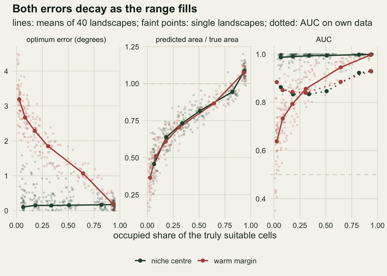
area_first    <- mar$area[1]
area_last     <- mar$area[n_stage]
area_mid      <- mar$area[4]
fill_mid      <- mar$fill[4]
opt_seq       <- abs(mar$opt - t_opt_true)
area_err_seq  <- abs(mar$area - 1)
mono_opt      <- all(diff(opt_seq) < 0)
mono_area     <- all(diff(area_err_seq) < 0)

## the same two questions asked of each landscape on its own
mono_count <- function(pl, v, target) {
  sum(vapply(seq_len(n_land), function(i) {
    sel <- runs$placement == pl & runs$land == i
    ser <- abs(runs[[v]][sel][order(runs$gen[sel])] - target)
    all(diff(ser) < 0)
  }, logical(1)))
}
mono_opt_n  <- mono_count("warm margin", "opt", t_opt_true)
mono_area_n <- mono_count("warm margin", "area", 1)
cen_area_first <- cen$area[1]
cen_area_last  <- cen$area[n_stage]
auc_true_first <- mar$auc_true[1]
auc_true_last  <- mar$auc_true[n_stage]
auc_true_min   <- min(runs$auc_true[runs$placement == "warm margin"])
mar_early      <- runs[runs$placement == "warm margin" & runs$gen == stage_gen[1], ]
auc_rev_n      <- sum(mar_early$auc_true < 0.5)
auc_rev_rate   <- auc_rev_n / n_land
auc_rev_se     <- sqrt(auc_rev_rate * (1 - auc_rev_rate) / n_land)
auc_true_early_min <- min(mar_early$auc_true)
area_r_last    <- mar$area_r[n_stage]
area_r_first   <- mar$area_r[1]
cen_area_r_last <- cen$area_r[n_stage]

## is the equilibrium area ratio a bullseye, or significantly above one?
mar_last     <- runs[runs$placement == "warm margin" & runs$gen == stage_gen[n_stage], ]
area_last_tt <- t.test(mar_last$area, mu = 1)
area_last_ci <- as.numeric(area_last_tt$conf.int)
sink_last    <- mar$sink_share[n_stage]
area_g_last  <- mar$area_g[n_stage]
area_g_first <- mar$area_g[1]
For the warm-margin introduction the predicted suitable area is 0.36 of the truth at 2.6 per cent fill, 0.70 at 30.6 per cent, and 1.07 at 93.3 per cent. The optimum error falls from 3.2 degrees to 0.2. Both mean sequences move towards the truth at every one of the 6 stages (mean optimum error decreasing at every step: yes; distance of the mean area ratio from one decreasing at every step: yes). Asked of each landscape on its own the answer is weaker: the optimum error falls at every step in 36 of the 40 warm-margin landscapes and the area ratio approaches one at every step in 24 of them, the rest wobbling at one step or another. The size of the error is a readout of how far the invasion has got, on average and not in every replicate, and nothing else changes between the panels.
The niche-centre introduction loses area on almost the same schedule, from 0.46 of the truth at the earliest stage to 1.08 at the last, with a mean optimum that was never wrong. Getting the response curve right does not protect the area, because the area is set by where the model puts its threshold and the threshold is calibrated on presences that all come from one part of the gradient.
AUC against the true suitable set does fall, from 1.00 at the last stage to 0.64 at the first, and on average it stays above a half: a model fitted to a young invasion usually still ranks suitable cells above unsuitable ones. The average hides the spread. At the earliest stage the 40 warm-margin landscapes gave values from 0.35 to 0.87, and 5 of the 40 were below a half, which is a ranking worse than a coin’s: a rate of 0.125 with a binomial standard error of 0.052. Whether the ranking reverses is a property of the landscape rather than of the invasion, and the honest limits below return to it.
What the threshold rule decides
Turning a fitted surface into an area needs a cut-off, and the two rules carried through the sweep disagree about the last stage. Under the relative rule, cells above 0.3 of the surface maximum, the warm-margin area ratio runs from 0.36 at the earliest stage to 1.25 at the last, with the niche-centre set ending at 1.25 as well. Under the tenth-percentile training-presence rule the same fits end at 1.07. A rule set relative to the surface maximum rewards a flat fitted surface, so a model fitted at a nearly full range over-predicts by about a quarter under it.
The percentile rule is nearer the truth at that stage but it is not on it. Its equilibrium mean of 1.075 has a 95 per cent interval of 1.061 to 1.089 over the 40 landscapes, which excludes one (t = 11.0 on 39 degrees of freedom). The overshoot is not an accident of the rule, and the Honest limits below give its cause.
The percentile rule also has a weakness at the young end of the sweep. At the earliest stage it is taken over 30 presence cells on average and as few as 9, and at that size the tenth percentile is barely distinguishable from the lowest fitted value at any presence, which is the rule Pearson and colleagues set out rather than the variant named above.
Reading the fitted quadratic itself as a suitability surface is not the threshold-free escape it looks like. Recentring the linear predictor on its own peak turns the fit into a Gaussian in temperature, and putting that through the same 0.3 cut-off gives an area ratio of 0.35 at the earliest stage and 0.64 at the last, where the range is 93 per cent full and the model is nearly right. That last number is not a model error: a fitted occupancy probability is a steeper function of temperature than suitability is, so the two surfaces are on different scales and the ratio between them never closes. The quantities that can be compared without a rule are the ranking ones, which is why AUC against the true suitable set is reported at every stage above.
So any statement about how much area an early model loses is a statement about a threshold rule as well as about the model, and the rule has to be quoted with the number.
An accessible-area background is not the repair
The accessible area of Barve and colleagues is the region the species could plausibly have reached, and restricting the model to it removes the absences that are absences only because dispersal has not delivered anything there. Implemented here as the obvious buffer: keep only cells within five cells of an occupied cell, refit the same quadratic, project onto the whole grid.
paired_gain <- function(v1, v0, pl) {
  out <- t(vapply(stage_gen, function(g) {
    sel <- runs$placement == pl & runs$gen == g
    d   <- runs[[v1]][sel] - runs[[v0]][sel]
    c(mean(d), sd(d) / sqrt(length(d)))
  }, numeric(2)))
  data.frame(gen = stage_gen, gain = out[, 1], se = out[, 2],
             t = out[, 1] / out[, 2])
}
gain_area <- paired_gain("area_buf", "area", "warm margin")
gain_auc  <- paired_gain("auc_tr_buf", "auc_true", "warm margin")
gain_r    <- paired_gain("area_r_buf", "area_r", "warm margin")
gain_auc_best <- gain_auc[which.max(gain_auc$gain), ]
missing_first <- 1 - mar$area[1]
share_first   <- mar$buf_share[1]
opt_buf_first <- mar$opt_buf[1]
At the earliest stage the buffer holds 20 per cent of the grid, and the refitted model gives a predicted area of 0.369 of the truth against 0.365 for the model fitted on every cell. Taken landscape by landscape rather than as a difference of means, that gain is 0.0044 of the truth with a paired standard error of 0.0043 over the 40 landscapes, so it is not distinguishable from no change at all, and at no stage of the sweep does the paired area gain reach two standard errors (the largest is 0.0101 at 1.7 standard errors). The area the young model was missing was 0.64 of the truth, and no measurable part of it comes back. Its fitted optimum, 19.1 degrees, sits 3.1 degrees from the truth against 3.2 for the model fitted on every cell, a shift too small to move any map.
The ranking does improve, slightly, and that is the main thing the buffer buys. AUC against the true suitable set gains 0.016 at the earliest stage (paired standard error 0.006) and 0.029 at generation 8, its best stage (paired standard error 0.008). Those gains are about three standard errors wide, so they are real, and they are also of a size that changes no decision: a model whose predicted extent is a third of the truth is not rescued by sorting cells a little better.
The reason is not subtle. The buffer removes the absences beyond the front, which is the right idea, but the presences are unchanged and they still all sit on one part of the gradient, so the fitted quadratic still has no information about the cool side of the niche. What the buffer removes is the evidence against the cool side, not the missing evidence for it. Under the relative threshold rule the buffer looks much better than this. It gains 0.051 of the truth at the earliest stage (paired standard error 0.009, 5.7 standard errors) against 0.0044 under the percentile rule, and the relative-rule gain is at its most certain in the middle of the sweep, 0.060 of the truth at generation 16 and 19.3 standard errors wide. The gain is real and it is the rule’s arithmetic rather than new information: a background restricted to a small buffer produces a flatter projected surface, and a threshold set relative to the surface maximum converts flatness into area. Anyone reporting an accessible-area repair under a relative rule is reporting that conversion.
The check you can run on your own records
The diagnostic follows from the mechanism. If the fitted optimum is the centre of the occupied cloud, and the occupied cloud early in an invasion is the founding site, then a fitted optimum that has not moved away from the climate of the earliest records is a fitted optimum that has learned nothing the founders did not already say. The quantity is the distance in climate space between the fitted optimum and the mean climate of the earliest records.
runs$found_gap <- abs(runs$opt - runs$temp_found)
gap_mean <- aggregate(cbind(found_gap, fill) ~ placement + gen, data = runs, FUN = mean)

ggplot(runs, aes(fill, found_gap, colour = placement)) +
  geom_hline(yintercept = 1, linetype = "dashed", colour = te_line,
             linewidth = 0.6) +
  geom_point(alpha = 0.35, size = 1.5) +
  geom_line(data = gap_mean, linewidth = 1.1) +
  geom_point(data = gap_mean, size = 2.6) +
  scale_colour_manual(values = c("warm margin" = te_rust,
                                 "niche centre" = te_forest), name = NULL) +
  labs(x = "occupied share of the truly suitable cells",
       y = "fitted optimum to founding climate (degrees)",
       title = "The distance grows only if the founders were off centre",
       subtitle = sprintf("points: single landscapes; lines: means of %d",
                          n_land)) +
  theme_datasheet() +
  theme(legend.position = "bottom",
        plot.margin = margin(5.5, 12, 5.5, 5.5))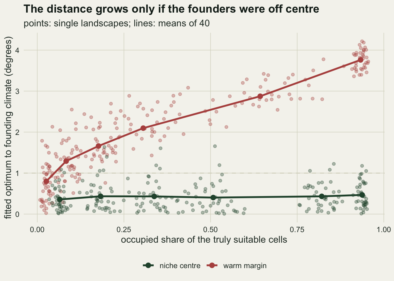
flag_cut   <- 1
early_rows <- runs[runs$gen == stage_gen[1], ]
late_rows  <- runs[runs$gen == stage_gen[n_stage], ]
flag_early <- sum(early_rows$found_gap < flag_cut)
n_each     <- nrow(early_rows)
flag_late_cen <- sum(late_rows$found_gap[late_rows$placement == "niche centre"] < flag_cut)
flag_late_mar <- sum(late_rows$found_gap[late_rows$placement == "warm margin"] < flag_cut)
flag_early_mar <- sum(early_rows$found_gap[early_rows$placement == "warm margin"] < flag_cut)
flag_early_cen <- sum(early_rows$found_gap[early_rows$placement == "niche centre"] < flag_cut)
gap_mar_rng_e <- range(early_rows$found_gap[early_rows$placement == "warm margin"])
gap_mar_rng_l <- range(late_rows$found_gap[late_rows$placement == "warm margin"])
area_late_cen_rng <- range(late_rows$area[late_rows$placement == "niche centre"])
area_early_rng    <- range(early_rows$area)
Across the warm-margin landscapes the distance is between 0.02 and 2.13 degrees at the earliest stage and between 3.36 and 4.21 degrees at the last. Those two sets do not overlap, so on this contrast the distance separates a model fitted to a young range from one fitted to a filled range without any reference to the truth.
The niche-centre landscapes are where the check fails, and it fails in a way that has to be stated with it. There the distance stays below 1.66 degrees at every stage, including the last, because the founding site happened to sit at the optimum and the fitted optimum has nowhere to travel. Taking a distance under 1 degree as a flag for “this model may be fitted to a young range”, a cut-off fixed before the sweep was run, the flag fires on 26 of the 40 warm-margin fits at the earliest stage and on 0 at the last, which is the wanted direction but only 65 per cent of the cases it was built for. On the niche-centre fits it fires 38 times of 40 at the earliest stage and 38 times at the last, where it means nothing at all. Two things follow. The flag at that cut-off is closer to a test of where the founding site sat than of how full the range is. And the cut-off is carrying weight that no truth-free rule can give it: the warm-margin distances at the two ends of the sweep do not overlap, so some cut separates them perfectly, but 1 degree is not that cut and nothing in the model output says where to put one.
So the check is one-sided, and that is its honest description. A large distance is informative: the model has learned something beyond the founding site, and the founding records are no longer driving the response. A small distance is not: it is consistent with a model that has learned nothing and with a model that is right for a species introduced into the middle of its niche. The two cases are separated by the other number, the occupied share, and by nothing in the model output. At the last stage the niche-centre fits had area ratios between 0.99 and 1.20, against 0.14 to 0.66 for the earliest-stage fits of both kinds, and the distance to the founding climate was under a degree in 38 of the 40 fits in the first group and 64 of the 80 in the second.
What to report
Report the occupied share of the accessible suitable area alongside any projected map, and be explicit that it is a guess. It is the quantity that decides how much of the error above applies, it is not in the model output, and a range known to be expanding is a range for which the projected area is a lower bound. The area ratios above are a rough scale: at a few per cent occupancy expect the projection to be a third to a half of the potential range, on this simulation’s parameters.
Report the distance between the fitted optimum and the climate of the earliest records, and report it as a one-sided check with the distance itself rather than a flag. If the distance is large, say so and move on. If it is small, the model output cannot distinguish a fit calibrated to the founding site from a correct fit for a species introduced into the middle of its niche, and the only thing that separates them is outside information: how much of the reachable suitable area is occupied, and whether the founding site is near the centre of the species’ range in its native area.
Quote the threshold rule with every area figure. The same fits at the same stages give an equilibrium area ratio of 1.07 under the tenth-percentile training presence rule, 1.25 under a rule relative to the surface maximum, and 0.64 if the fitted quadratic is read as a suitability surface instead. A reader who is handed an area without a rule has been handed a number that cannot be checked.
Do not report an internal AUC as evidence about the niche. On these simulations it stayed between 0.84 and 0.93 while the predicted area went from 0.36 of the truth to 1.07. If a discrimination measure is reported at all, it should be on a spatial split, which is what Spatial cross-validation for SDMs in R is about, and even that measures ranking rather than extent.
If an accessible-area background is used, say what it changed. Here it changed the area by 0.0044 of the truth against a paired standard error of 0.0043, that is by nothing measurable, and the optimum by 0.09 degrees against a bias of 3.2 degrees; it improved the ranking by 0.016 of AUC, which is measurable and small. It is a defensible choice about which question the model answers, in the sense that the pseudo-absence post gives it, and it is not a correction for a species that has not finished spreading.
Honest limits
The occupied set never becomes the truly suitable set, not even at the last stage, so the area ratio does not have one as its target. At generation 40 of the warm-margin runs, 15 per cent of the presences sit in cells whose suitability is below the cut-off, held there by colonisation from suitable neighbours: with eight occupied neighbours the colonisation probability at a suitability of 0.1 is 0.25 against an extinction probability of 0.14, so sink occupancy is built into the process. A model fitted to that occupied set is fitted to something slightly larger than the suitable set, which is why the equilibrium area ratio of 1.075 sits significantly above one rather than landing on it. Read the right-hand end of the area panel as the process’s own equilibrium, not as a bullseye.
The simulation has one climate variable, and the fitted model has the matching quadratic. Real models have several correlated covariates, and the front is then a direction in that space rather than a point on an axis. The founding-climate check generalises to a distance in covariate space, but the scale of that distance is not the scale measured here, and a Mahalanobis-type distance in a correlated set behaves differently from degrees on one axis.
The absences are perfect. Every cell was visited, every occupied cell was found, and the only reason for a zero is the species’ absence. Add imperfect detection and the model is fitted to a further-shrunken presence set, which moves everything in the same direction as the bias measured here. The interaction is not measured above, and the occupancy posts on this site are where that problem belongs.
The earliest records are treated as a known quantity. They are not: they are the output of a search process, and Checking an unstructured-data analysis measures how much effort moves a first record, with the farthest sites in that example getting a small fraction of the effort the nearest ones get. If the first records come from ports, gardens and botanic collections, their climate is partly a statement about where people look. The check compares the fitted optimum with those records, so it inherits their bias, and in the common case where recording effort and the introduction point are in the same warm, lowland, populated places the two biases point the same way and the check will understate the problem.
AUC against the true suitable set reversed, that is fell below a half, in 5 of the 40 warm-margin landscapes at the earliest stage and in none at any later stage, a rate of 0.12 with a binomial standard error of 0.05, and a minimum over the whole set of 0.35. How far it falls depends on how much warm unsuitable and cool unsuitable land the map holds, because the fitted quadratic ranks the warm unsuitable cells above the cool unsuitable ones and the two classes have different sizes in different landscapes; here there were 2.8 warm unsuitable cells to every cool one on average, and a generator with the opposite asymmetry would give a different rate. That is a property of the landscape’s composition rather than of the invasion, so the mean of 0.64 at the earliest stage should be read as this landscape generator’s number and not as a general rate.
The introduction contrast is two points, not a gradient. The warm-margin and niche-centre cases bracket the range of behaviour, but the interesting quantity, how the size of the error depends on how far the founding climate sits from the optimum, would need a sweep over that distance rather than two values of it.
The spread process has no long-distance dispersal. Colonisation only reaches the eight neighbours, so the occupied set stays compact and the front stays sharp. Jumps ahead of the front put presences into climates the compact process would not have reached, which weakens the correlation between absence and climate and therefore reduces the bias; Long-distance jumps and stratified spread and Fat tails and accelerating spread cover the spread side of that. Similarly, no spatial smoother was fitted here: a term in the coordinates can absorb part of the dispersal structure, and what it does to the climatic response is a separate question from the one measured above.
The area ratios rest on a single true-suitability cut-off of 0.3 and on 40 landscapes. The Monte Carlo standard errors are small relative to the large effects, 0.017 on the earliest-stage area ratio, though not relative to the small ones: the buffer’s area gain above never reaches twice its own standard error at any stage, and that is the reason it is reported as no gain rather than as a small one. The definition of the true suitable set is also a modelling choice: a stricter cut-off gives a smaller denominator and a larger ratio at every stage, without changing the shape of the curve against fill.
References
Vaclavik T, Meentemeyer RK 2012 Diversity and Distributions 18(1):73-83 (10.1111/j.1472-4642.2011.00854.x)
Barve N, Barve V, Jimenez-Valverde A, Lira-Noriega A, Maher SP, Peterson AT, Soberon J, Villalobos F 2011 Ecological Modelling 222(11):1810-1819 (10.1016/j.ecolmodel.2011.02.011)
Elith J, Kearney M, Phillips S 2010 Methods in Ecology and Evolution 1(4):330-342 (10.1111/j.2041-210X.2010.00036.x)
Pearson RG, Raxworthy CJ, Nakamura M, Peterson AT 2007 Journal of Biogeography 34(1):102-117 (10.1111/j.1365-2699.2006.01594.x)