library(ggplot2)

te_pal <- list(forest = "#275139", green = "#2f8f63", sage = "#93a87f",
               clay = "#b5534e", gold = "#cda23f", line = "#dad9ca",
               ink = "#16241d", paper = "#f5f4ee")

theme_te <- function() {
  theme_minimal(base_size = 12) +
    theme(panel.grid.minor = element_blank(),
          panel.grid.major = element_line(colour = "#e7e6dc"),
          plot.background = element_rect(fill = "#f5f4ee", colour = NA),
          panel.background = element_rect(fill = "#f5f4ee", colour = NA),
          plot.title = element_text(face = "bold", colour = te_pal$ink),
          axis.title = element_text(colour = "#2c3a31"))
}Checking an unstructured-data analysis
R
citizen science
monitoring
ecology tutorial
ggplot2
Four checks on a trend built from opportunistic records in R: effort in space and time, reporting bias between species, first records, and external validation.
A county records centre holds twenty years of lists. Somebody walked a site, wrote down what they saw and sent it in. Nobody allocated the site, nobody timed the visit, and nobody was asked to report what was absent. The target species appears on a rising share of those lists, the graph goes up and to the right, and the county report says the species is recovering. In the dataset built below that reading is exactly wrong: the species is losing 5.4 per cent of its occupancy odds every year and the record stream reports it gaining 3.0 per cent, because the observers changed faster than the species did.
The three earlier posts in this cluster build the machinery that is supposed to prevent this. List-length analysis for opportunistic data treats the number of species on a submitted list as a measure of how hard the observer looked, and conditions the trend on it. Reporting rates and effort drift measures how large a false trend a change in observer behaviour can manufacture on its own, and separates the kinds of drift that produce it. Occupancy from unstructured records constructs repeat visits out of the record stream so that a detection model can be fitted to them. All three return an estimate with an interval, and the intervals are narrow, because opportunistic datasets are large.
That effort corrupts a trend is not news on this blog. First flowering date and sampling effort shows it on a phenological extreme and sampling bias in presence-only models shows the same confound laid out in space rather than time. What follows is not a fifth demonstration of the confound. It is four measurements of what the corrections for it achieve and what they leave behind, run on a simulator whose answer is fixed before any model is fitted: a spatial correction and a temporal one applied to the same records, two species with an identical decline and different reputations, the year of a first record, and the smallest structured survey that can catch the whole thing out. Where a check comes back saying the correction did less than advertised, that is the result and it stays in.
The record stream under test
One simulator carries three of the four checks. The landscape is sixty sites arranged along a single habitat axis, from unsuitable at one end to good at the other. The target species occupies a site with a probability that depends on that axis and on the year: the log odds fall by 0.055 every year at every site, which is the quantity every estimator below is trying to find. Occupancy is redrawn each year rather than carried forward, so the trend is a clean logistic drift with no colonisation and extinction dynamics underneath it.
A visit is one person going to one site on one day and submitting the list of what they found. The visit has an effort, drawn on a log scale, and the chance of recording the target given that it is present rises with effort along an exponential detection curve. Sixty other species make up the rest of the list. Their occupancy is drawn independently of the habitat axis that drives the target, which is deliberate: it makes the length of a list a measure of effort and nothing else, so that the two biases in check 1 can be separated. Real lists are not this obliging, and that matters later.
Two knobs generate the drift. The first raises the average effort per visit as the years pass, which is the temporal mechanism: better optics and more patient recorders. The second tilts the choice of site towards the good end of the habitat axis, which is the spatial mechanism: observers learn where the species is and go there. Both can be switched off, which is what makes the yardstick in check 1 possible. Everything here assumes the records have already been through the sort of tidying in Cleaning GBIF occurrence data; none of the defects below is a data quality problem, and none of them can be cleaned away.
set.seed(20260805)

n_years  <- 20
n_sites  <- 60
vis_year <- 110
q_site   <- seq(-1.5, 1.5, length.out = n_sites)
yr_mid   <- (n_years + 1) / 2

beta_true <- -0.055
psi_int   <- -0.40
psi_hab   <- 1.20
lam_tar   <- 0.85
eff_lm    <- log(0.9)
eff_ls    <- 0.40

n_bg   <- 60
u_bg   <- runif(n_bg, 0.15, 0.85)
lam_bg <- runif(n_bg, 0.10, 0.70)

tau_on   <- 0.045
kappa_on <- 0.06

sim_unstr <- function(tau, kappa, n_vis = vis_year) {
  yr  <- rep(seq_len(n_years), each = n_vis)
  n_v <- length(yr)
  site <- integer(n_v)
  for (tt in seq_len(n_years)) {
    w <- exp(kappa * (tt - 1) * q_site)
    site[yr == tt] <- sample.int(n_sites, n_vis, replace = TRUE, prob = w)
  }
  eff <- exp(rnorm(n_v, eff_lm + tau * (yr - 1), eff_ls))
  lp  <- outer(psi_int + psi_hab * q_site, beta_true * (seq_len(n_years) - yr_mid), "+")
  z   <- matrix(rbinom(n_sites * n_years, 1, plogis(lp)), n_sites, n_years)
  y   <- z[cbind(site, yr)] * rbinom(n_v, 1, 1 - exp(-lam_tar * eff))
  occ_bg <- matrix(rbinom(n_sites * n_bg, 1, rep(u_bg, each = n_sites)), n_sites, n_bg)
  det_bg <- matrix(rbinom(n_v * n_bg, 1, 1 - exp(-outer(eff, lam_bg))), n_v, n_bg)
  list(y = y, yr = yr - yr_mid, year = yr, q = q_site[site], eff = eff,
       ll = log(rowSums(det_bg * occ_bg[site, ]) + 1))
}

beta_of <- function(d, cols) {
  X <- cbind(1, d$yr)
  if ("ll"  %in% cols) X <- cbind(X, d$ll)
  if ("q"   %in% cols) X <- cbind(X, d$q)
  if ("eff" %in% cols) X <- cbind(X, log(d$eff))
  glm.fit(X, d$y, family = binomial())$coefficients[2]
}

c(years = n_years, sites = n_sites, visits_per_year = vis_year,
  total_visits = n_years * vis_year, background_species = n_bg)
years sites visits_per_year total_visits
20 60 110 2200
background_species
60 round(c(true_trend_log_odds = beta_true,
occupancy_worst_site_year_one = plogis(psi_int + psi_hab * min(q_site) -
beta_true * (yr_mid - 1)),
occupancy_best_site_year_one = plogis(psi_int + psi_hab * max(q_site) -
beta_true * (yr_mid - 1)),
effort_growth_over_study = exp(tau_on * (n_years - 1)),
site_preference_ratio_final_year = exp(kappa_on * (n_years - 1) *
diff(range(q_site)))), 3) true_trend_log_odds occupancy_worst_site_year_one
-0.055 0.157
occupancy_best_site_year_one effort_growth_over_study
0.872 2.351
site_preference_ratio_final_year
30.569 round(c(true_odds_change_percent = 100 * (exp(beta_true) - 1)), 1)true_odds_change_percent
-5.4 d_demo <- sim_unstr(tau_on, kappa_on)
c(records_of_target = sum(d_demo$y))records_of_target
760 round(c(mean_list_length = mean(exp(d_demo$ll) - 1),
list_length_year_one = mean(exp(d_demo$ll[d_demo$year == 1]) - 1),
list_length_final_year = mean(exp(d_demo$ll[d_demo$year == n_years]) - 1),
effort_variance_explained = summary(lm(log(d_demo$eff) ~ d_demo$ll))$r.squared,
good_site_share_year_one = mean(d_demo$q[d_demo$year == 1] > 0.5),
good_site_share_final_year = mean(d_demo$q[d_demo$year == n_years] > 0.5)), 3) mean_list_length list_length_year_one
14.313 9.836
list_length_final_year effort_variance_explained
18.900 0.648
good_site_share_year_one good_site_share_final_year
0.327 0.755 With both knobs on, twenty years of recording produce 2200 lists carrying 760 records of the target. The lists get longer as the study runs, from a mean of 9.836 species in the first year to 18.900 in the last, and the log of list length explains 0.648 of the variance in log effort, which is the reason list length is used as a proxy at all. The visits also move: 0.327 of them land on the better third of the gradient in the first year and 0.755 in the last. In the final year a visit is 30.569 times more likely to fall on the best site than on the worst, and effort per visit has grown by a factor of 2.351. Neither figure is extreme next to what the large recording platforms have actually done in twenty years.
That is a dataset an analyst would be pleased to receive. It has thousands of lists, a clear covariate for effort, and a species whose occupancy runs from 0.157 at the poor end of the gradient to 0.872 at the good end in the first year. Everything below is done on it.
Check 1: two biases, two corrections
Two things drift in this record stream and they drift for unrelated reasons. Observers spend longer per visit as the years pass, so the chance of recording a species that is present rises even where nothing has changed. Observers also learn where the good sites are, so the visits migrate up the habitat gradient, which raises the reporting rate for a species that likes the good end. Both look like a recovery on a graph of records per list. Neither is one.
The check crosses four record-generating scenarios with five model specifications. The scenarios are no drift, effort drift in time only, drift in site choice only, and both together. The specifications are a bare year term, year plus log list length, year plus the site habitat covariate, year plus both, and year plus the true per-visit effort alongside the habitat term, which no analyst ever has and which is included to show what the proxy costs. Each cell is the mean over 120 replicate datasets.
The comparison needs a yardstick and the true occupancy trend is the wrong one. A reporting rate is occupancy multiplied by detection, and the year coefficient of a reporting rate is smaller in size than the year coefficient of the occupancy underneath it, before any drift is involved at all. So each specification is judged against its own value in the no-drift scenario. The first column of the second table below is that yardstick, which is why it is a column of zeros.
set.seed(20260805)
n_rep1 <- 120

scen <- list(none = c(0, 0), temporal = c(tau_on, 0),
             spatial = c(0, kappa_on), both = c(tau_on, kappa_on))
est <- list(none = character(0), list = "ll", habitat = "q",
            both = c("ll", "q"), effort = c("eff", "q"))

grid1 <- array(NA_real_, c(length(est), length(scen), n_rep1))
for (s in seq_along(scen)) for (r in seq_len(n_rep1)) {
  d <- sim_unstr(scen[[s]][1], scen[[s]][2])
  grid1[, s, r] <- vapply(est, function(e) beta_of(d, e), numeric(1))
}
mean1 <- apply(grid1, 1:2, mean)
sd1   <- apply(grid1, 1:2, sd)
dimnames(mean1) <- dimnames(sd1) <- list(names(est), names(scen))
bias1 <- mean1 - mean1[, "none"]

c(replicates = n_rep1)
replicates
120 print(round(mean1, 4)) none temporal spatial both
none -0.0319 -0.0039 -0.0036 0.0299
list -0.0323 -0.0214 -0.0037 0.0099
habitat -0.0346 -0.0048 -0.0328 -0.0006
both -0.0352 -0.0247 -0.0333 -0.0234
effort -0.0355 -0.0396 -0.0338 -0.0388print(round(bias1, 4)) none temporal spatial both
none 0 0.0279 0.0282 0.0617
list 0 0.0109 0.0286 0.0421
habitat 0 0.0299 0.0018 0.0340
both 0 0.0105 0.0018 0.0118
effort 0 -0.0041 0.0018 -0.0032print(round(sd1, 4)) none temporal spatial both
none 0.0112 0.0107 0.0118 0.0118
list 0.0112 0.0118 0.0119 0.0123
habitat 0.0120 0.0113 0.0124 0.0124
both 0.0120 0.0117 0.0125 0.0125
effort 0.0122 0.0125 0.0126 0.0129round(c(benchmark_uncorrected = mean1["none", "none"],
naive_estimate_both_drifts = mean1["none", "both"]), 4) benchmark_uncorrected naive_estimate_both_drifts
-0.0319 0.0299 removed <- function(row, col) 100 * (1 - bias1[row, col] / bias1["none", col])
round(c(attenuation_percent = 100 * mean1["none", "none"] / beta_true,
naive_odds_change_percent = 100 * (exp(mean1["none", "both"]) - 1),
temporal_removed_by_list = removed("list", "temporal"),
spatial_removed_by_list = removed("list", "spatial"),
spatial_removed_by_habitat = removed("habitat", "spatial"),
temporal_removed_by_habitat = removed("habitat", "temporal"),
both_removed_by_both = removed("both", "both"),
both_removed_by_true_effort = removed("effort", "both")), 1) attenuation_percent naive_odds_change_percent
57.9 3.0
temporal_removed_by_list spatial_removed_by_list
61.0 -1.3
spatial_removed_by_habitat temporal_removed_by_habitat
93.5 -7.0
both_removed_by_both both_removed_by_true_effort
80.9 105.3 est_lab <- c(none = "year only", list = "plus list length", habitat = "plus habitat",
both = "plus both", effort = "plus true effort and habitat")
scen_lab <- c(none = "no drift", temporal = "effort drift in time",
spatial = "drift in site choice", both = "both drifts")
grid_df <- data.frame(
scenario = factor(rep(scen_lab[colnames(mean1)], each = nrow(mean1)),
levels = scen_lab),
spec = factor(rep(est_lab[rownames(mean1)], ncol(mean1)), levels = est_lab),
fit = as.vector(mean1), sdv = as.vector(sd1))
ggplot(grid_df, aes(scenario, fit, colour = spec)) +
geom_hline(yintercept = 0, colour = "#9c9c90", linetype = "12", linewidth = 0.5) +
geom_hline(yintercept = beta_true, colour = te_pal$ink, linewidth = 0.6) +
geom_linerange(aes(ymin = fit - sdv, ymax = fit + sdv),
position = position_dodge(width = 0.62), linewidth = 0.7) +
geom_point(position = position_dodge(width = 0.62), size = 2.6) +
annotate("text", x = 0.45, y = 0.003, label = "no trend", hjust = 0, vjust = 0,
size = 3.1, colour = "#7d7d72") +
annotate("text", x = 0.45, y = beta_true - 0.003, label = "truth", hjust = 0,
vjust = 1, size = 3.1, fontface = "bold", colour = te_pal$ink) +
expand_limits(y = beta_true - 0.010) +
scale_y_continuous(expand = expansion(mult = c(0.07, 0.08))) +
scale_colour_manual(values = c(te_pal$clay, te_pal$gold, te_pal$sage,
te_pal$green, te_pal$forest), name = NULL) +
guides(colour = guide_legend(nrow = 2)) +
labs(x = NULL, y = "Estimated trend in log odds per year",
title = "Each correction is blind to the other one's bias") +
theme_te() +
theme(legend.position = "top")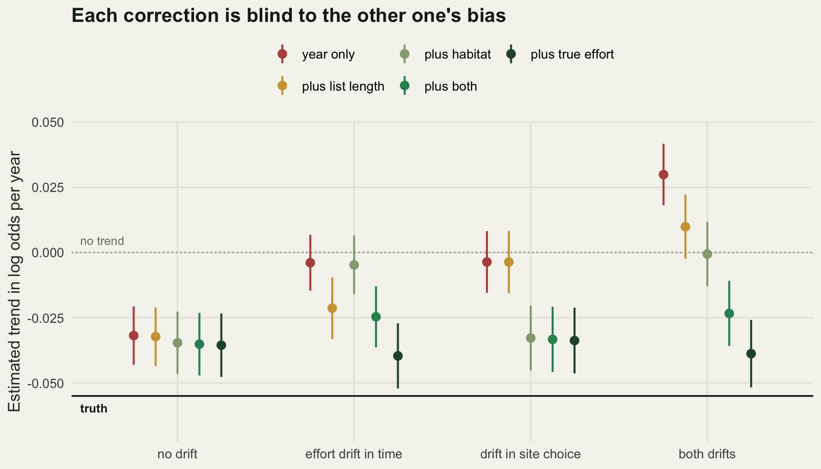
Start with the yardstick, because it is a result in its own right. With no drift at all, the bare year term returns -0.0319 against a true occupancy trend of -0.055, or 57.9 per cent of it. No correction in this post removes that gap, and no correction should: detection is imperfect, occupancy varies from site to site, and the log odds of a reporting rate move less than the log odds of the occupancy they come from. A trend fitted to opportunistic records is a trend in reports. Quoted as a rate of decline it will read as too slow, by a factor that depends on how detectable the species is and on how uneven the landscape is. The sign and the ordering survive; the magnitude does not.
Now the drift. With both mechanisms running, the bare year term returns +0.0299, so a species losing 5.4 per cent of its occupancy odds a year is reported as gaining 3.0 per cent. The bias is +0.0617 on a scale where the entire true signal is 0.055. It is larger than the thing being measured and it points the other way, and the replicate to replicate spread of 0.0118 means it is not going to be rescued by a longer time series either.
The rest of the table is the point of the check. The list length term removes 61.0 per cent of the bias generated by effort drift in time, and nothing at all of the bias generated by drift in site choice: the measured figure there is -1.3 per cent, which is zero plus noise. The habitat term is the mirror image. It removes 93.5 per cent of the spatial bias and -7.0 per cent of the temporal one, meaning it leaves the temporal problem very slightly worse than it found it. Each correction is close to invisible to the other one’s mechanism, and applying only one of them leaves a residual of 0.0421 or 0.0340, the first large enough on its own to reverse the reported sign and the second to erase the trend.
Applying both removes 80.9 per cent and leaves 0.0118. That remainder is the price of the proxy, not a fault of the approach: the specification handed the true per-visit effort removes 105.3 per cent, which is complete within Monte Carlo error. Log list length explains 0.648 of the variance in log effort in this dataset, and the part of the effort signal that the proxy does not carry is what comes back as the shortfall in the correction. A list length corrected trend is a partly effort corrected trend, and the size of the part that is missing is set by how well lists happen to track effort in that particular dataset. That is measurable if the effort is recorded on even a subset of visits, and it is worth measuring before the correction is described as done.
One practical note before the next check. The habitat covariate did the spatial work here because the simulator put the spatial structure on a single axis that the analyst was handed. In a real dataset the equivalent move is either a site level term, which costs degrees of freedom and needs sites to be revisited, or the target-group background trick from sampling bias in presence-only models, which uses records of similar species to describe where the effort went. The next check is about what happens when that second idea is applied to the wrong problem.
Check 2: two species, one trend, two answers
A records database does not hold species. It holds reports of species, and between the animal and the row in the table sits a person deciding whether this one is worth writing down and whether they are sure enough of the name. That decision differs between species and it changes over time, and unlike effort it leaves no trace in the length of the list.
Two damselflies share this landscape. Both decline at exactly the same rate, the same 0.055 in occupancy log odds per year that check 1 was chasing. The first is large and unmistakable and gets written down 0.700 of the times it is seen, in the first year and in the last. The second is small and brown and needs a photograph and a key, so early in the study it is written down 0.289 of the times it is seen, rising to 0.650 by the final year as cameras get cheaper and the county recorder starts accepting photographs. Nothing about the animal changed. The recording culture around it did.
Eight further species share the second damselfly’s identification problem and its improvement. They are the reference group: the “similar species” that a records analyst would normalise against, on the reasoning that whatever inflates the target’s record count over time will inflate theirs by the same factor and cancel in the ratio. The third estimator below does exactly that, taking the target’s records each year as a share of the target plus reference records and fitting a trend to the share.
Effort is held constant in this check and the site choice is uniform, so nothing from check 1 is operating. The list length covariate is built from the sixty background species, whose reporting habits never change, so the identification improvement cannot leak into it. That separation is artificial and it is generous to the list length correction: in a real dataset improving identification lengthens the lists as well.
set.seed(20260805)
n_rep2 <- 80
n_ref  <- 8

u_ref   <- runif(n_ref, 0.30, 0.70)
lam_ref <- runif(n_ref, 0.25, 0.60)
rho_a   <- 0.70
rho_b   <- function(tt) plogis(-0.9 + 0.08 * (tt - 1))

sim_taxon <- function(drift) {
  yr  <- rep(seq_len(n_years), each = vis_year)
  n_v <- length(yr)
  site <- sample.int(n_sites, n_v, replace = TRUE)
  eff  <- exp(rnorm(n_v, eff_lm, eff_ls))
  lp   <- outer(psi_int + psi_hab * q_site, beta_true * (seq_len(n_years) - yr_mid), "+")
  pdet <- 1 - exp(-lam_tar * eff)
  za <- matrix(rbinom(n_sites * n_years, 1, plogis(lp)), n_sites, n_years)
  zb <- matrix(rbinom(n_sites * n_years, 1, plogis(lp)), n_sites, n_years)
  rb <- if (drift) rho_b(yr) else rho_b(yr_mid)
  ya <- za[cbind(site, yr)] * rbinom(n_v, 1, pdet) * rbinom(n_v, 1, rho_a)
  yb <- zb[cbind(site, yr)] * rbinom(n_v, 1, pdet) * rbinom(n_v, 1, rb)
  occ_ref <- matrix(rbinom(n_sites * n_ref, 1, rep(u_ref, each = n_sites)),
                    n_sites, n_ref)
  det_ref <- matrix(rbinom(n_v * n_ref, 1, (1 - exp(-outer(eff, lam_ref))) * rb),
                    n_v, n_ref)
  yref <- as.integer(rowSums(det_ref * occ_ref[site, ]) > 0)
  occ_bg <- matrix(rbinom(n_sites * n_bg, 1, rep(u_bg, each = n_sites)), n_sites, n_bg)
  det_bg <- matrix(rbinom(n_v * n_bg, 1, 1 - exp(-outer(eff, lam_bg))), n_v, n_bg)
  list(ya = ya, yb = yb, yref = yref, year = yr, yr = yr - yr_mid,
       ll = log(rowSums(det_bg * occ_bg[site, ]) + 1))
}

b_rate  <- function(y, d) glm.fit(cbind(1, d$yr), y, family = binomial())$coefficients[2]
b_list  <- function(y, d) glm.fit(cbind(1, d$yr, d$ll), y,
                                  family = binomial())$coefficients[2]
b_ratio <- function(y, d) {
  nt <- as.numeric(tapply(y, d$year, sum))
  nr <- as.numeric(tapply(d$yref, d$year, sum))
  glm.fit(cbind(1, seq_len(n_years) - yr_mid), nt / (nt + nr),
          weights = nt + nr, family = binomial())$coefficients[2]
}

tax <- lapply(c(FALSE, TRUE), function(dr) {
  set.seed(20260805)
  m <- vapply(seq_len(n_rep2), function(r) {
    d <- sim_taxon(dr)
    c(b_rate(d$ya, d), b_list(d$ya, d), b_ratio(d$ya, d),
      b_rate(d$yb, d), b_list(d$yb, d), b_ratio(d$yb, d))
  }, numeric(6))
  rownames(m) <- c("A rate", "A list", "A ratio", "B rate", "B list", "B ratio")
  m
})
mean2 <- cbind(steady = rowMeans(tax[[1]]), improving = rowMeans(tax[[2]]))
sd2   <- cbind(steady = apply(tax[[1]], 1, sd), improving = apply(tax[[2]], 1, sd))

c(replicates = n_rep2, reference_species = n_ref)
replicates reference_species
80 8 round(c(reporting_conspicuous = rho_a, reporting_overlooked_year_one = rho_b(1),
reporting_overlooked_final_year = rho_b(n_years)), 3) reporting_conspicuous reporting_overlooked_year_one
0.700 0.289
reporting_overlooked_final_year
0.650 print(round(cbind(mean2, bias = mean2[, "improving"] - mean2[, "steady"],
sd_improving = sd2[, "improving"]), 4)) steady improving bias sd_improving
A rate -0.0314 -0.0314 0.0000 0.0127
A list -0.0315 -0.0315 0.0000 0.0127
A ratio -0.0262 -0.0574 -0.0312 0.0115
B rate -0.0286 0.0199 0.0484 0.0148
B list -0.0286 0.0201 0.0486 0.0148
B ratio -0.0254 -0.0124 0.0130 0.0144round(c(gap_between_species_rate = mean2["B rate", "improving"] -
mean2["A rate", "improving"],
ratio_bias_added_to_conspicuous = mean2["A ratio", "improving"] -
mean2["A ratio", "steady"],
gap_after_ratio = mean2["B ratio", "improving"] -
mean2["A ratio", "improving"]), 4) gap_between_species_rate ratio_bias_added_to_conspicuous
0.0513 -0.0312
gap_after_ratio
0.0449 round(c(overlooked_odds_change_percent = 100 * (exp(mean2["B rate", "improving"]) - 1),
ratio_removed_from_overlooked = 100 * (1 -
(mean2["B ratio", "improving"] - mean2["B ratio", "steady"]) /
(mean2["B rate", "improving"] - mean2["B rate", "steady"])),
gap_closed_by_ratio = 100 * (1 -
(mean2["B ratio", "improving"] - mean2["A ratio", "improving"]) /
(mean2["B rate", "improving"] - mean2["A rate", "improving"]))), 1)overlooked_odds_change_percent ratio_removed_from_overlooked
2.0 73.2
gap_closed_by_ratio
12.3 sp_lab <- c(A = "conspicuous species", B = "overlooked species")
mt_lab <- c(rate = "reporting rate", list = "list length", ratio = "reference ratio")
parts <- do.call(rbind, strsplit(rownames(mean2), " ", fixed = TRUE))
tax_df <- data.frame(
species = factor(rep(sp_lab[parts[, 1]], 2), levels = sp_lab),
method = factor(rep(mt_lab[parts[, 2]], 2), levels = mt_lab),
panel = factor(rep(c("Reporting effort steady", "Identification improving"),
each = nrow(mean2)),
levels = c("Reporting effort steady", "Identification improving")),
fit = as.vector(mean2), sdv = as.vector(sd2))
ann_tax <- data.frame(panel = factor(levels(tax_df$panel)[1],
levels = levels(tax_df$panel)))
ggplot(tax_df, aes(method, fit, colour = species)) +
geom_hline(yintercept = 0, colour = "#9c9c90", linetype = "12", linewidth = 0.5) +
geom_hline(yintercept = beta_true, colour = te_pal$ink, linewidth = 0.6) +
geom_linerange(aes(ymin = fit - sdv, ymax = fit + sdv),
position = position_dodge(width = 0.5), linewidth = 0.7) +
geom_point(position = position_dodge(width = 0.5), size = 2.9) +
geom_text(data = ann_tax, aes(x = 0.45, y = 0.004, label = "no trend"),
inherit.aes = FALSE, hjust = 0, vjust = 0, size = 3.1,
colour = "#7d7d72") +
geom_text(data = ann_tax, aes(x = 0.45, y = beta_true - 0.004, label = "truth"),
inherit.aes = FALSE, hjust = 0, vjust = 1, size = 3.1,
fontface = "bold", colour = te_pal$ink) +
expand_limits(y = beta_true - 0.012) +
scale_y_continuous(expand = expansion(mult = c(0.07, 0.06))) +
facet_wrap(~panel) +
scale_colour_manual(values = c(te_pal$forest, te_pal$clay), name = NULL) +
labs(x = NULL, y = "Estimated trend in log odds per year",
title = "The same decline is reported two different ways") +
theme_te() +
theme(legend.position = "top",
strip.text = element_text(colour = te_pal$ink, face = "bold"))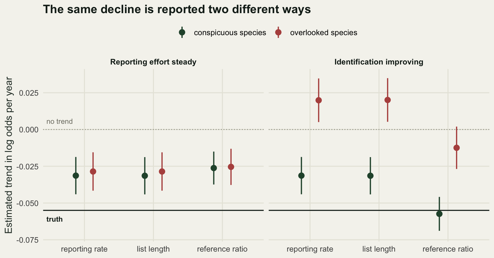
The conspicuous species is reported as declining at -0.0314. The overlooked one, declining at the same true rate in the same landscape in the same years, is reported as increasing at +0.0199, or 2.0 per cent in odds per year. The gap between them is 0.0513, which is close to the size of the true trend both of them share. Two species, one decline, and a difference in the answer nearly as large as the signal, produced entirely by who bothered to write them down.
The list length correction does not touch it. The overlooked species goes from +0.0199 to +0.0201, and the conspicuous one from -0.0314 to -0.0315. This is the expected result rather than a failure, and it is worth saying out loud because the two ideas are easy to run together: list length measures how hard the observer looked, and says nothing about whether the observer could name what they were looking at. The check 1 correction is the right instrument pointed at the wrong defect.
The reference ratio is the standard defence and it half works. It removes 73.2 per cent of the overlooked species’ bias, bringing it from +0.0484 down to +0.0130 and back below zero to -0.0124, which is at least the right sign. It also injects -0.0312 into the conspicuous species, whose reporting propensity never moved: that estimate goes from -0.0262 with steady reporting to -0.0574 with the reference group improving, a decline more than twice as steep as the same estimator returns when nothing drifts, and now spuriously close to the true occupancy trend. The ratio did not delete a bias. It moved the reference group’s drift into the answer for whatever sits in the numerator, with the sign reversed.
The measurement that settles it is the gap. Before normalising, two identically declining species differ by 0.0513. After normalising, they differ by 0.0449. The reference ratio closed 12.3 per cent of the discrepancy it was introduced to remove, and rearranged the rest. What it actually estimates is the target’s trend minus the reference group’s trend, which is the quantity you want only when two things hold at once: the reference group’s reporting drift matches the target’s, and the reference group has no real trend of its own. Neither is checkable inside the same dataset, because a group of species whose reporting is drifting is exactly the group whose apparent trend cannot be trusted.
There is a practical rule in here. Where the reference group is chosen for taxonomic convenience, which is usually how it is chosen, the ratio is a bet that the whole genus or family shares one recording history and one ecological fate. Where the reference group is chosen because its members share an identification difficulty with the target and are known from other evidence to be stable, the ratio is a reasonable correction. The second kind of reference group is far harder to assemble, and the difference between the two is invisible in the output.
Check 3: the first record is an effort statistic
Trends are averages and averages are forgiving. The first record is not: it is a single extreme order statistic, it is quoted to the day or the year in almost every account of an arriving species, and it is the input to every estimate of how fast something is spreading. First flowering date and sampling effort measured what effort does to the first date of a phenological season. The same arithmetic applies to the first year of an occupancy, and the consequences are worse, because the spread rate is a slope fitted through a set of first records rather than a single one.
The setting changes for this check. A species arrives at one point in year 2 of a twenty-five year study and spreads outward from there at 11 kilometres a year. Forty sites lie along the line of advance, from 5 to 200 kilometres out. Once the front passes a site, the species holds it with probability 0.85 in any given year. Visits arrive as a Poisson stream and each visit has a fixed chance of finding the species if it is there.
Two questions follow. How much later is the same arrival detected when there is less recording, and what does the pattern of recording do to the fitted speed? Three effort patterns are compared at the same total number of visits: constant, growing through time at a rate that multiplies effort by 9.850 over the study, and falling with distance from the introduction point so that the farthest sites get 0.062 of the effort the nearest ones get. That last one is not a contrivance. Recorders live where the people are, and introductions usually start there.
set.seed(20260805)
n_rep3 <- 300
n_yr_c <- 25
n_st_c <- 40

d_km    <- seq(5, 200, length.out = n_st_c)
v_true  <- 11
arrive0 <- 2
a_true  <- arrive0 + d_km / v_true
psi_est <- 0.85
p_vis   <- 1 - exp(-lam_tar * 0.9)
yrs_c   <- seq_len(n_yr_c)
occ_ok  <- outer(a_true, yrs_c, function(a, tt) as.numeric(tt >= a))

first_rec <- function(rate) {
  vis <- matrix(rpois(length(rate), rate), n_st_c, n_yr_c)
  occ <- occ_ok * matrix(rbinom(n_st_c * n_yr_c, 1, psi_est), n_st_c, n_yr_c)
  hit <- matrix(rbinom(n_st_c * n_yr_c, 1, occ * (1 - (1 - p_vis)^vis)),
                n_st_c, n_yr_c)
  apply(hit, 1, function(r) if (any(r == 1)) which(r == 1)[1] else NA_real_)
}
flat_rate <- function(m) matrix(m, n_st_c, n_yr_c)
grow_rate <- function(m, g) {
  w <- g^(yrs_c - 1)
  flat_rate(m) * rep(w / mean(w), each = n_st_c)
}
near_rate <- function(m, sc) {
  w <- exp(-d_km / sc)
  flat_rate(m) * (w / mean(w))
}

rate_grid <- c(0.25, 0.5, 1, 2, 4)
lag_rate <- vapply(rate_grid, function(m)
  mean(replicate(n_rep3, mean(first_rec(flat_rate(m)) - a_true, na.rm = TRUE))),
  numeric(1))
names(lag_rate) <- paste0("visits_", rate_grid)

base_rate <- 1.5
growth_g  <- 1.10
near_sc   <- 70
gens <- list(constant = function() first_rec(flat_rate(base_rate)),
             growing  = function() first_rec(grow_rate(base_rate, growth_g)),
             near_end = function() first_rec(near_rate(base_rate, near_sc)))
speed <- vapply(gens, function(g) {
  z <- replicate(n_rep3, {
    f <- g()
    ok <- !is.na(f)
    c(1 / coef(lm(f[ok] ~ d_km[ok]))[2], sum(ok))
  })
  c(speed = mean(z[1, ]), sd = sd(z[1, ]), sites = mean(z[2, ]))
}, numeric(3))

c(replicates = n_rep3, sites = n_st_c, study_years = n_yr_c)
replicates sites study_years
300 40 25 round(c(true_speed_km_per_year = v_true, nearest_site_km = min(d_km),
farthest_site_km = max(d_km), occupancy_behind_the_front = psi_est,
visits_per_site_year = base_rate,
effort_growth_over_study = growth_g^(n_yr_c - 1),
far_site_effort_share = exp(-diff(range(d_km)) / near_sc)), 3) true_speed_km_per_year nearest_site_km
11.000 5.000
farthest_site_km occupancy_behind_the_front
200.000 0.850
visits_per_site_year effort_growth_over_study
1.500 9.850
far_site_effort_share
0.062 print(round(lag_rate, 3))visits_0.25 visits_0.5 visits_1 visits_2 visits_4
5.279 3.723 2.163 1.242 0.787 print(round(speed, 3)) constant growing near_end
speed 11.040 12.986 9.518
sd 0.483 0.953 0.492
sites 39.867 39.993 36.687round(c(lag_saved_by_effort = unname(lag_rate[1] - lag_rate[length(lag_rate)]),
sites_missed_near = unname(n_st_c - speed["sites", "near_end"])), 3)lag_saved_by_effort sites_missed_near
4.492 3.313 round(c(speed_error_growing_percent = unname(100 * (speed["speed", "growing"] /
v_true - 1)),
speed_error_near_percent = unname(100 * (speed["speed", "near_end"] /
v_true - 1))), 1)speed_error_growing_percent speed_error_near_percent
18.1 -13.5 set.seed(20260805)
fr_show <- data.frame(
dist = rep(d_km, 3),
year = c(first_rec(flat_rate(base_rate)), first_rec(grow_rate(base_rate, growth_g)),
first_rec(near_rate(base_rate, near_sc))),
effort = rep(c("constant effort", "effort grows in time",
"effort falls with distance"), each = n_st_c))
c(sites_without_a_record_in_this_replicate = sum(is.na(fr_show$year)))sites_without_a_record_in_this_replicate
3 fr_show <- fr_show[!is.na(fr_show$year), ]eff_lab <- c("constant effort", "effort grows in time", "effort falls with distance")
fr_show$effort <- factor(fr_show$effort, levels = eff_lab)
truth_line <- data.frame(dist = range(d_km), year = arrive0 + range(d_km) / v_true)
ggplot(fr_show, aes(dist, year, colour = effort)) +
geom_line(data = truth_line, aes(dist, year), inherit.aes = FALSE,
colour = te_pal$ink, linetype = "22", linewidth = 0.7) +
annotate("text", x = 148, y = arrive0 + 148 / v_true - 0.7,
label = "true colonisation year", hjust = 0, vjust = 1,
size = 3.2, fontface = "bold", colour = te_pal$ink) +
geom_point(size = 2.2, alpha = 0.85) +
geom_smooth(method = "lm", formula = y ~ x, se = FALSE, linewidth = 0.9) +
scale_colour_manual(values = c(te_pal$forest, te_pal$clay, te_pal$gold), name = NULL) +
labs(x = "Distance from the point of introduction (km)",
y = "Year of first record",
title = "Growing effort makes the spread look faster than it is") +
theme_te() +
theme(legend.position = "top")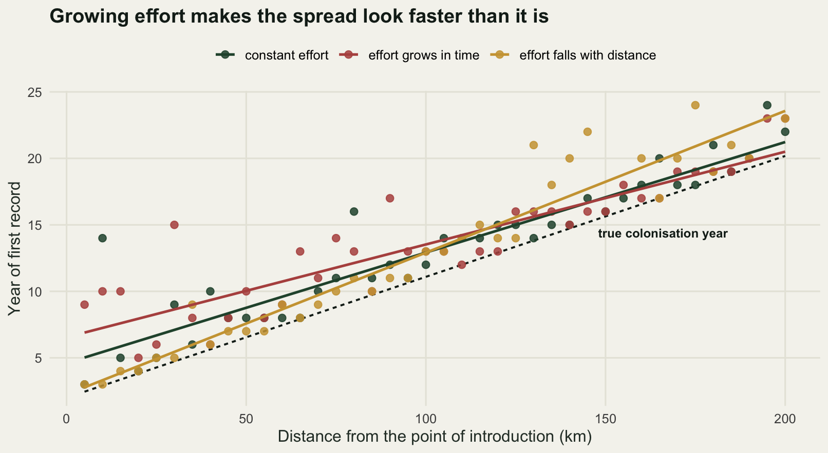
The detection lag is large and it is a pure function of effort. At a quarter of a visit per site per year the average first record arrives 5.279 years after the species does. At four visits per site per year it arrives 0.787 years after. The same colonisation, in the same landscape, with the same detectability, is dated 4.492 years apart by the recording intensity alone. A dated first record is a statement about recorders as much as about the species, and comparing first records between a well watched county and a poorly watched one mostly compares the counties.
The spread rate is where it becomes expensive. With constant effort the regression of first record year on distance recovers 11.040 kilometres a year against a true 11, because the lag is roughly the same at every site and disappears into the intercept. Turn on effort that grows through time and the estimate rises to 12.986, an error of 18.1 per cent. The mechanism is worth following: the distant sites are colonised late, late is when the recording is dense, so distant sites carry a shorter lag than near ones. The observed arrival dates are compressed towards each other, the fitted slope of years against distance is too shallow, and the invasion looks faster than it is. Growth in recording effort and the outward progress of an invasion are confounded by construction, because both are functions of time.
Effort that falls with distance from the introduction point does the opposite and gives 9.518, an error of -13.5 per cent, because the far sites now wait longer than the near ones for their first record. It also quietly deletes data: an average of 3.313 of the forty sites are never recorded at all within the study, and 3 in the replicate plotted above, so the regression is fitted to the part of the front that was watched. The two biases are of similar size and opposite sign, and a real recording scheme has both running at once, which means the net error on a published spread rate is not signed in advance. The spread of the estimate across replicates is also about twice as large under growing effort, 0.953 against 0.483, so the confidence interval that comes with the biased figure is wider as well as wrong.
None of this is fixed by a list length correction, and it is not clear what would fix it short of modelling the recording process and the invasion together. The cheap partial defence is to estimate the spread from the change in occupied area over time, using all the records rather than the first one at each site, since that estimator uses the middle of the distribution instead of its extreme edge.
Check 4: what the structured survey is for
The first three checks are internal. They compare specifications against each other on the same records, and every one of them would run happily on a dataset whose bias nobody had noticed. This one comes from outside: a structured survey, meaning sites picked by the analyst rather than by the observer, visited three times a year with the same protocol every year. It costs money, and it is the only thing here that can measure the bias rather than assume it.
Three estimators go on the table. The unstructured analysis with the list length correction only, which is the common practice case: the effort proxy is used because it is easy and the spatial term is left out because site is not always recorded well enough to include. The unstructured analysis with both corrections, which from check 1 carries a small residual bias. And the structured survey alone, at sample sizes from four sites up to a census of all sixty. Errors are measured against what the same reporting-rate estimator returns from that census, which comes out at -0.0317, in agreement with check 1’s no-drift benchmark of -0.0319. The two datasets are then pooled by inverse variance weighting, which is the simplest way anyone combines two independent estimates of the same quantity.
The first question is how much structured survey it takes to catch the unstructured analysis out. The test is the ordinary two-sample comparison of the two trend estimates against their combined standard error, at the 0.05 level, and the power is the share of the 150 replicates in which it fires.
set.seed(20260805)
n_rep4 <- 150
n_str_visit <- 3
eff_str <- 0.9
k_grid <- c(4, 8, 16, 24, 32, 60)

sim_str <- function() {
  sj <- rep(seq_len(n_sites), each = n_years * n_str_visit)
  st <- rep(rep(seq_len(n_years), each = n_str_visit), n_sites)
  lp <- outer(psi_int + psi_hab * q_site, beta_true * (seq_len(n_years) - yr_mid), "+")
  z  <- matrix(rbinom(n_sites * n_years, 1, plogis(lp)), n_sites, n_years)
  list(y = z[cbind(sj, st)] * rbinom(length(sj), 1, 1 - exp(-lam_tar * eff_str)),
       yr = st - yr_mid, site = sj)
}
beta_se <- function(X, y) {
  f <- glm.fit(X, y, family = binomial())
  rr <- f$qr$qr[seq_len(ncol(X)), seq_len(ncol(X)), drop = FALSE]
  rr[lower.tri(rr)] <- 0
  c(f$coefficients[2], sqrt(diag(chol2inv(rr)))[2])
}

val <- t(vapply(seq_len(n_rep4), function(r) {
  d  <- sim_unstr(tau_on, kappa_on)
  u1 <- beta_se(cbind(1, d$yr, d$ll), d$y)
  u2 <- beta_se(cbind(1, d$yr, d$ll, d$q), d$y)
  s  <- sim_str()
  ord <- sample(n_sites)
  z <- vapply(k_grid, function(k) {
    sel <- s$site %in% ord[seq_len(k)]
    beta_se(cbind(1, s$yr[sel]), s$y[sel])
  }, numeric(2))
  c(u1, u2, as.vector(z))
}, numeric(4 + 2 * length(k_grid))))
colnames(val) <- c("u1", "u1se", "u2", "u2se",
                   paste0(rep(c("k", "se"), length(k_grid)),
                          rep(k_grid, each = 2)))

yard <- mean(val[, "k60"])
pool <- function(bu, su, bs, ss) {
  w <- (1 / su^2) / (1 / su^2 + 1 / ss^2)
  w * bu + (1 - w) * bs
}
rmse <- function(x) sqrt(mean((x - yard)^2))
vtab <- t(vapply(seq_along(k_grid), function(i) {
  bs <- val[, paste0("k", k_grid[i])]
  ss <- val[, paste0("se", k_grid[i])]
  c(sites = k_grid[i], structured = rmse(bs), nominal_se = mean(ss),
    spread = sd(bs), pooled = rmse(pool(val[, "u2"], val[, "u2se"], bs, ss)),
    pooled_uncorrected = rmse(pool(val[, "u1"], val[, "u1se"], bs, ss)),
    power = mean(abs(val[, "u1"] - bs) / sqrt(val[, "u1se"]^2 + ss^2) > 1.96))
}, numeric(7)))

c(replicates = n_rep4, structured_visits_per_site_year = n_str_visit)
replicates structured_visits_per_site_year
150 3 round(c(yardstick = yard, no_drift_benchmark = mean1["none", "none"],
unstructured_list_only = mean(val[, "u1"]),
unstructured_list_only_bias = mean(val[, "u1"]) - yard,
unstructured_both = mean(val[, "u2"]),
unstructured_both_bias = mean(val[, "u2"]) - yard,
unstructured_both_rmse = rmse(val[, "u2"]),
unstructured_list_only_rmse = rmse(val[, "u1"]),
unstructured_nominal_se = mean(val[, "u2se"]),
unstructured_spread = sd(val[, "u2"])), 4) yardstick no_drift_benchmark
-0.0317 -0.0319
unstructured_list_only unstructured_list_only_bias
0.0113 0.0430
unstructured_both unstructured_both_bias
-0.0207 0.0110
unstructured_both_rmse unstructured_list_only_rmse
0.0170 0.0448
unstructured_nominal_se unstructured_spread
0.0094 0.0130 print(round(vtab, 4)) sites structured nominal_se spread pooled pooled_uncorrected power
[1,] 4 0.0343 0.0279 0.0343 0.0154 0.0407 0.4133
[2,] 8 0.0244 0.0194 0.0245 0.0145 0.0373 0.5600
[3,] 16 0.0169 0.0135 0.0170 0.0130 0.0323 0.7133
[4,] 24 0.0145 0.0110 0.0146 0.0118 0.0283 0.7733
[5,] 32 0.0123 0.0096 0.0123 0.0104 0.0250 0.8400
[6,] 60 0.0086 0.0070 0.0086 0.0083 0.0183 0.9333c(structured_sites_beating_unstructured =
k_grid[which(vtab[, "structured"] < rmse(val[, "u2"]))[1]])structured_sites_beating_unstructured
16 round(c(pooled_rmse_at_four_sites = unname(vtab[1, "pooled"])), 4)pooled_rmse_at_four_sites
0.0154 round(c(pooled_gain_at_four_sites_percent =
unname(100 * (1 - vtab[1, "pooled"] / rmse(val[, "u2"]))),
pooled_gain_at_census_percent =
unname(100 * (1 - vtab[nrow(vtab), "pooled"] /
vtab[nrow(vtab), "structured"])),
nominal_se_share_four_sites_percent =
unname(100 * vtab[1, "nominal_se"] / vtab[1, "spread"]),
nominal_se_share_unstructured_percent =
100 * mean(val[, "u2se"]) / sd(val[, "u2"])), 1) pooled_gain_at_four_sites_percent pooled_gain_at_census_percent
9.6 4.0
nominal_se_share_four_sites_percent nominal_se_share_unstructured_percent
81.3 72.4 val_lab <- c("structured survey alone", "corrected unstructured alone",
"the two pooled", "pooled without the habitat term")
val_df <- rbind(
data.frame(k = k_grid, rmse = vtab[, "structured"], src = val_lab[1]),
data.frame(k = k_grid, rmse = rmse(val[, "u2"]), src = val_lab[2]),
data.frame(k = k_grid, rmse = vtab[, "pooled"], src = val_lab[3]),
data.frame(k = k_grid, rmse = vtab[, "pooled_uncorrected"], src = val_lab[4]))
val_df$src <- factor(val_df$src, levels = val_lab)
ggplot(val_df, aes(k, rmse, colour = src, shape = src)) +
geom_line(linewidth = 0.9) +
geom_point(size = 2.7, stroke = 1.1, fill = NA) +
scale_x_log10(breaks = k_grid, labels = k_grid) +
scale_colour_manual(values = c(te_pal$clay, te_pal$gold, te_pal$forest,
te_pal$sage), name = NULL) +
scale_shape_manual(values = c(21, 22, 24, 23), name = NULL) +
guides(colour = guide_legend(nrow = 2), shape = guide_legend(nrow = 2)) +
labs(x = "Structured survey sites", y = "Root mean squared error of the trend",
title = "Pooling helps most while the structured survey is small") +
theme_te() +
theme(legend.position = "top")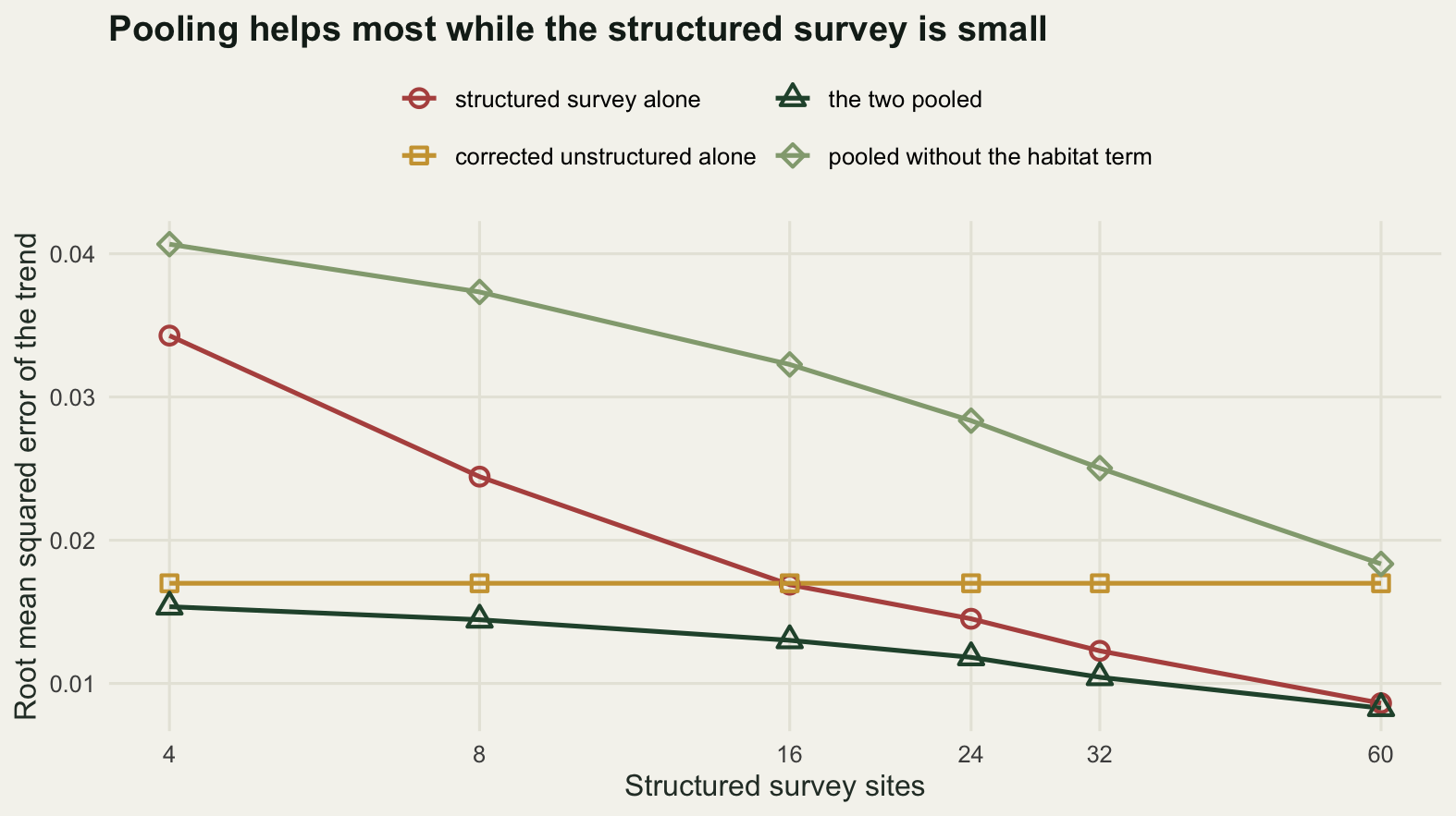
The bias being hunted is large: the list length only analysis returns +0.0113 against a yardstick of -0.0317, so it has the sign wrong and misses by 0.0430. Four structured sites detect that in 0.4133 of replicates, eight in 0.5600, sixteen in 0.7133, and thirty-two in 0.8400. A survey of half the landscape, run every year for twenty years, is what it takes here to be reasonably sure of catching an error that reverses the direction of the published trend. Anyone who has budgeted a validation survey as a small add-on to a records project should sit with that number for a moment. It is also the optimistic version, for a reason that appears two paragraphs below.
The second measurement is the one that changes how the two datasets should be talked about. The corrected unstructured analysis has a root mean squared error of 0.0170: a residual bias of +0.0110 from the imperfect effort proxy, plus a spread of 0.0130 from ordinary sampling noise. The structured survey is unbiased by construction here, but it is small, and its error at four sites is 0.0343 and at eight sites 0.0244. Both are worse than the biased unstructured analysis. Sixteen structured sites is where the structured survey first wins on its own here, at 0.0169 against 0.0170. Below that, the clean small survey is the less accurate of the two, and a project that discards its opportunistic records on the grounds that they are biased has thrown away the better estimate.
Pooling beats both here at every sample size on the table, though the margin over the structured survey narrows to nothing at the top end. At four structured sites the pooled error is 0.0154, which is 9.6 per cent better than the corrected unstructured analysis on its own and less than half the structured survey’s own error. At the census of sixty sites the pooled error is 4.0 per cent below the structured survey’s own, a margin small enough to be noise, since by then the structured data carry most of the weight. The shape of that curve is the useful part: the marginal value of a structured site is highest when there are almost none, and a validation survey does not need to be big enough to stand alone to be worth running. Its job is to hold the unstructured analysis in place, not to replace it.
The pooling has one condition and the fourth line on the figure is what happens without it. Pooling the uncorrected analysis, the one with the list length term and no spatial term, gives an error of 0.0407 at four sites and 0.0183 at the census: worse than the structured survey alone at every sample size, and worse than doing nothing at all with the records. Inverse variance weighting has no defence against bias. It gives the largest weight to the estimate with the smallest standard error, and a large biased dataset has a very small standard error. Combining datasets is only an improvement once the biased one has been corrected to the point where its remaining bias is small next to the other one’s noise, and check 1 is how you find out whether it has been.
One warning about all the standard errors in this section, which applies to the power figures above as well. The visit level binomial model treats every visit as independent, and visits at the same site in the same year are not: they share one occupancy state. The nominal standard error is 81.3 per cent of the true spread for the four-site structured survey and 72.4 per cent for the corrected unstructured analysis. Both intervals are too narrow, in the dataset and in the direction that makes an analysis look more settled than it is. The detection powers quoted above are therefore too high, since the test that produced them used those understated errors.
The honest limit
The simulator was built to make the four checks separable, and the separations are the part that would not survive contact with a real records database.
The clearest of them is in check 1. The sixty species that set the list length have occupancy drawn independently of the habitat axis the target responds to, which is what makes list length a measure of effort and nothing else. Let the background species prefer the same good sites and the list length term starts absorbing part of the spatial drift as well, which sounds like good news and is not: the two mechanisms then share a covariate, the correction for one becomes a partial correction for the other, and the tidy accounting of what was removed and by which term stops being available. The same collapse happens in check 2 if improving identification lengthens the lists, which in the field it certainly does.
Occupancy is redrawn every year, independently, so there is no colonisation and extinction process and no persistence in the pattern of occupied sites. That makes the true trend exactly the logistic drift written into the simulator, and it makes the estimators look better behaved than they would be against a real metapopulation, where this year’s occupancy is mostly last year’s. Check 4’s standard errors are already too narrow by about a quarter from within-site correlation alone, and site persistence across years would widen that gap further.
The estimand is a reporting-rate trend throughout, and check 1 measured how far that sits from the occupancy trend: 57.9 per cent of it here, with a factor that depends on detectability and on how uneven occupancy is across the landscape. None of the corrections in this post recovers the occupancy scale, which is what the occupancy model in Occupancy from unstructured records is for, and which brings its own assumptions. If the output is going to be quoted as a percentage change per year, this is the step where the number is decided.
Last, and least fixable: every check here compares a correction against a bias that was put into the simulator deliberately. A bias that is constant in time, constant in space and the same for every species does not move any of these four estimates at all, and none of the checks can see it. The whole apparatus is built to detect changes in observer behaviour. A recording culture that has always been wrong in the same way passes every one of them.
Where to go next
Three of the four checks are cheap enough to run on any records dataset before the trend is written up. Check 1 needs one extra covariate and a comparison of specifications, and the useful output is not the corrected estimate but the distance between the corrected and uncorrected ones. Check 2 needs a second species with a known trend, or failing that, an honest statement of which direction the target’s reporting culture has moved. Check 3 needs nothing at all beyond a decision not to build a spread rate out of first records. Only check 4 costs money, and the measurement there is that a small validation survey buys more than its own precision would suggest.
For the machinery being tested, List-length analysis for opportunistic data is where the effort proxy is built and its functional form chosen, and Reporting rates and effort drift separates the kinds of observer change that produce the bias measured in check 1. If the attenuation in the first check is the part that matters for your question, meaning you need a rate of change rather than a direction, Occupancy from unstructured records is the route to an estimate on the occupancy scale. And for the design side of check 4, on how many sites and how many years buy how much power in a survey you control, Checking a survey design does that arithmetic from the other end.
References
Isaac NJB, van Strien AJ, August TA, de Zeeuw MP, Roy DB 2014 Methods in Ecology and Evolution 5(10):1052-1060 (10.1111/2041-210X.12254)
van Strien AJ, van Swaay CAM, Termaat T 2013 Journal of Applied Ecology 50(6):1450-1458 (10.1111/1365-2664.12158)
Boakes EH, McGowan PJK, Fuller RA, Chang-qing D, Clark NE, O’Connor K, Mace GM 2010 PLoS Biology 8(6):e1000385 (10.1371/journal.pbio.1000385)
Phillips SJ, Dudik M, Elith J, Graham CH, Lehmann A, Leathwick J, Ferrier S 2009 Ecological Applications 19(1):181-197 (10.1890/07-2153.1)
Szabo JK, Vesk PA, Baxter PWJ, Possingham HP 2010 Ecological Applications 20(8):2157-2169 (10.1890/09-0877.1)
MacKenzie DI, Nichols JD, Lachman GB, Droege S, Royle JA, Langtimm CA 2002 Ecology 83(8):2248-2255 (10.1890/0012-9658(2002)083[2248:ESORWD]2.0.CO;2)