library(ggplot2)

te_pal <- list(forest = "#275139", green = "#2f8f63", sage = "#93a87f",
               clay = "#b5534e", gold = "#cda23f", line = "#dad9ca",
               ink = "#16241d", paper = "#f5f4ee")

theme_te <- function() {
  theme_minimal(base_size = 12) +
    theme(panel.grid.minor = element_blank(),
          panel.grid.major = element_line(colour = "#e7e6dc"),
          plot.background = element_rect(fill = "#f5f4ee", colour = NA),
          panel.background = element_rect(fill = "#f5f4ee", colour = NA),
          plot.title = element_text(face = "bold", colour = te_pal$ink),
          axis.title = element_text(colour = "#2c3a31"))
}Occupancy from unstructured records
R
citizen science
monitoring
ecology tutorial
ggplot2
Turn opportunistic species records into repeat visits, fit an occupancy model in R by hand, and measure how much the definition of a visit moves the estimate.
A county recording scheme hands you a single summer of data: eighteen thousand records, each one a species, a date, a place and a recorder, and not one of them collected to a design. Someone on the committee wants to know what share of the county the target species actually occupies, and they have read enough to know that the answer is not the share of cells it was seen in, because nobody searched most of the county and plenty of those who did would have walked past the animal anyway.
Occupancy models exist for exactly that question, and they want something the database does not appear to contain: repeat visits to fixed sites, so that the pattern of detections and blanks at a site can separate absence from failure to detect. The database has no visits. It has records. But a record is evidence that somebody was standing somewhere at some time with their eyes open, and if you are willing to say that two records from the same place within some span of time came from the same search, you can build a detection history out of a record stream. This post builds one, and then measures the price: how much the estimate moves when the span of time, the size of the place and the loyalty of the recorders change, on data where the right answer is known.
The likelihood is not the new part. Single-season occupancy model writes the MacKenzie likelihood out by hand and maximises it with optim on data from a designed survey, and the same function, the same two parameters and the same call appear below without modification. Everything that changes sits upstream of the model, in the step that turns records into histories. The other route through the same problem, keeping the records as records and conditioning on list length in a regression, is list-length analysis for opportunistic data.
A season of records with a known answer
The county is a rectangle of one kilometre cells, 48 across and 24 down. The target species occupies a fixed 0.30 of them, laid out as a smooth field crossed with fine grain noise rather than scattered at random, because real distributions are patchy at several scales at once and the patch structure matters later. Seventy recorders each make around 36 trips over a 90 day season. A trip is one recorder, one cell, one morning, lasting three hours, and it produces a handful of records of whatever else was about plus, if the cell is occupied and the recorder is lucky, one record of the target. Detection is 0.35 per trip.
Two features of the design are deliberate. Each recorder has a home cell drawn uniformly over the county and wanders a short distance from it, so effort is heavily clumped in space but the clumps are not placed with any regard to the species: the cells that end up with records are not a biased sample of occupancy, which keeps the spatial sampling problem out of the way of the question being asked here. And no recorder makes two trips to the same cell on the same day, which gives the visit reconstruction a target it could in principle hit exactly.
grid_x <- 48; grid_y <- 24
n_cells <- grid_x * grid_y
season_days <- 90
trip_hours <- 3
n_obs <- 70
trips_mean <- 36
home_sd <- 1.2
list_rate <- 6
p_base <- 0.35
psi_target <- 0.30
cell_x <- ((seq_len(n_cells) - 1) %% grid_x) + 1
cell_y <- ((seq_len(n_cells) - 1) %/% grid_x) + 1
print(c(cells_across = grid_x, cells_down = grid_y, base_cells = n_cells,
        season_days = season_days, hours_per_trip = trip_hours, recorders = n_obs,
        mean_trips_each = trips_mean, mean_extra_records = list_rate))
cells_across cells_down base_cells season_days
48 24 1152 90
hours_per_trip recorders mean_trips_each mean_extra_records
3 70 36 6 print(c(true_detection = p_base, true_occupancy = psi_target))true_detection true_occupancy
0.35 0.30 make_field <- function() {
fld <- numeric(n_cells)
for (k in 1:5) {
fx <- runif(1, 0.6, 2.2); fy <- runif(1, 0.6, 2.2); ph <- runif(1, 0, 2 * pi)
fld <- fld + sin(2 * pi * (fx * cell_x / grid_x + fy * cell_y / grid_y) + ph)
}
zz <- fld / sd(fld) + rnorm(n_cells, 0, 0.55)
as.numeric(zz > quantile(zz, 1 - psi_target))
}
simulate_trips <- function() {
occ <- make_field()
home <- sample.int(n_cells, n_obs, replace = TRUE)
n_per <- pmax(rpois(n_obs, trips_mean), 4L)
who <- rep(seq_len(n_obs), n_per)
n_trip <- length(who)
tx <- pmin(pmax(round(cell_x[home][who] + rnorm(n_trip, 0, home_sd)), 1), grid_x)
ty <- pmin(pmax(round(cell_y[home][who] + rnorm(n_trip, 0, home_sd)), 1), grid_y)
day <- unlist(lapply(n_per, function(k) sample.int(season_days, k)))
list(occ = occ, n_trip = n_trip, obs = who, cell = (ty - 1) * grid_x + tx,
day = day, start = (day - 1) * 24 + runif(n_trip, 6, 13))
}
trip_p <- function(tr, skill_sd = 0, shuffle = FALSE) {
if (skill_sd <= 0) return(list(p = rep(p_base, tr$n_trip), obs = tr$obs))
who <- if (shuffle) sample(tr$obs) else tr$obs
sk <- rnorm(n_obs, 0, skill_sd)[who]
b <- uniroot(function(z) mean(plogis(z + sk)) - p_base, c(-9, 9))$root
list(p = plogis(b + sk), obs = who)
}
background <- function(tr, share = 1, extra = list_rate) {
nb <- rbinom(tr$n_trip, 1L, share) * (1L + rpois(tr$n_trip, extra))
idx <- rep(seq_len(tr$n_trip), nb)
list(trip = idx, time = tr$start[idx] + runif(length(idx), 0, trip_hours))
}
assemble <- function(tr, bg, pv, seen) {
hit <- which(seen)
trip <- c(bg$trip, hit)
tm <- c(bg$time, tr$start[hit] + runif(length(hit), 0, trip_hours))
ord <- order(tm)
list(trip = trip[ord], time = tm[ord],
tgt = c(rep(0, length(bg$trip)), rep(1, length(hit)))[ord],
cell = tr$cell[trip][ord], obs = pv$obs[trip][ord],
n_trip = tr$n_trip, occ = tr$occ)
}
set.seed(20260804)
tr <- simulate_trips()
pv <- trip_p(tr)
bg <- background(tr)
rc <- assemble(tr, bg, pv, tr$occ[tr$cell] > 0 & runif(tr$n_trip) < pv$p)
print(c(occupied_cells = sum(tr$occ), trips = tr$n_trip, records = length(rc$trip),
target_records = sum(rc$tgt), cells_with_records = length(unique(rc$cell)))) occupied_cells trips records target_records
346 2558 18009 282
cells_with_records
797 round(c(realised_occupancy = mean(tr$occ),
share_of_county_with_records = length(unique(rc$cell)) / n_cells,
records_per_trip = length(rc$trip) / tr$n_trip,
trips_in_the_busiest_cell = max(table(tr$cell))), 4) realised_occupancy share_of_county_with_records
0.3003 0.6918
records_per_trip trips_in_the_busiest_cell
7.0403 19.0000 The season produces 2558 trips and 18009 records, of which 282 are the target species. Records reach 797 cells, so 0.6918 of the county has been looked at by somebody, and the busiest single cell was walked 19 times. Occupancy is 0.3003 in this particular landscape, and detection is 0.35 per trip. Both are known throughout, which is the only reason any of the numbers below mean anything.
The likelihood does not change, only the data step
A visit history is a pair of numbers per site: how many visits, and how many of them found the species. Constructing one from records means choosing a key that says which records belong to the same visit, then collapsing the records within each key. Everything interesting in this post is a choice of key.
The model that consumes those histories is the standard single-season one. A site is occupied with probability psi; if it is occupied, each of its K visits detects the species independently with probability p. A site with at least one detection contributes psi times the binomial term. A site with none contributes the mixture of an occupied site missed K times and an unoccupied site. Both parameters are estimated on the logit scale with optim, and the standard errors come from the Hessian through the delta method.
histories <- function(site_rec, key_rec, tgt_rec) {
  uk <- unique(key_rec)
  f <- match(key_rec, uk)
  vdet <- as.vector(rowsum(tgt_rec, f)) > 0
  vsite <- site_rec[match(uk, key_rec)]
  us <- unique(vsite)
  g <- match(vsite, us)
  list(site = us, K = as.vector(rowsum(rep(1, length(vdet)), g)),
       Y = as.vector(rowsum(as.numeric(vdet), g)))
}

occ_nll <- function(par, K, Y) {
  psi <- min(max(plogis(par[1]), 1e-9), 1 - 1e-9)
  p   <- min(max(plogis(par[2]), 1e-9), 1 - 1e-9)
  ll <- ifelse(Y > 0, log(psi) + Y * log(p) + (K - Y) * log1p(-p),
               log(psi * exp(K * log1p(-p)) + 1 - psi))
  -sum(ll)
}

fit_occ <- function(K, Y) {
  st <- qlogis(c(min(max(mean(Y > 0), 0.05), 0.95),
                 min(max(sum(Y) / sum(K), 0.05), 0.95)))
  fo <- optim(st, occ_nll, K = K, Y = Y, method = "BFGS", hessian = TRUE)
  vc <- try(solve(fo$hessian), silent = TRUE)
  se <- if (inherits(vc, "try-error")) c(NA_real_, NA_real_) else sqrt(pmax(diag(vc), 0))
  ps <- plogis(fo$par)
  c(psi = ps[1], p = ps[2], se_psi = ps[1] * (1 - ps[1]) * se[1],
    se_p = ps[2] * (1 - ps[2]) * se[2])
}

visit_key <- function(rec, w, use_obs) {
  kk <- rec$cell * 4096 + floor(rec$time / w)
  if (use_obs) kk * 128 + rec$obs else kk
}

h_true <- histories(rc$cell, rc$trip, rc$tgt)
h_cdo  <- histories(rc$cell, visit_key(rc, 24, TRUE), rc$tgt)
print(c(same_sites = identical(h_true$site, h_cdo$site),
        same_visit_counts = identical(h_true$K, h_cdo$K),
        same_detections = identical(h_true$Y, h_cdo$Y)))
same_sites same_visit_counts same_detections
TRUE TRUE TRUE print(head(data.frame(cell = h_true$site, visits = h_true$K, detections = h_true$Y,
occupied = rc$occ[h_true$site]), 6)) cell visits detections occupied
1 265 1 0 1
2 6 7 3 1
3 943 6 0 0
4 1029 7 0 0
5 817 19 6 1
6 693 1 0 0round(c(sites = length(h_true$K), visits = sum(h_true$K),
mean_visits_per_site = mean(h_true$K),
share_of_sites_visited_once = mean(h_true$K == 1),
naive_occupancy = mean(h_true$Y > 0),
occupancy_of_cells_with_records = mean(rc$occ[h_true$site])), 4) sites visits
797.0000 2558.0000
mean_visits_per_site share_of_sites_visited_once
3.2095 0.2748
naive_occupancy occupancy_of_cells_with_records
0.2045 0.3212 print(round(fit_occ(h_true$K, h_true$Y), 4)) psi p se_psi se_p
0.3207 0.3432 0.0246 0.0218 Start with the calibration case, the one that has to work before anything else is worth reading. Group records by cell, by day and by recorder. Because no recorder visits a cell twice in a day, that key recovers the real trips exactly: same sites, same visit counts, same detections, all three checks true. The 18009 records collapse to 2558 visits over 797 sites, 3.2095 visits per site, with 0.2748 of the sites carrying only one visit.
The species was seen in 0.2045 of those sites and actually occupies 0.3212 of them. The model returns 0.3207 with a standard error of 0.0246, and a detection probability of 0.3432 against a true 0.35 with a standard error of 0.0218. A record stream with no design behind it has put occupancy at 0.3207 where the truth is 0.3212, while the count of cells with a sighting would have said 0.2045. That is the whole promise of the approach, and it holds because the visit reconstruction was exact.
Nothing else in this post is exact.
busy <- as.integer(names(sort(table(tr$cell), decreasing = TRUE))[1])
rules <- c(0, 1, 24, 168, 672)
rule_lab <- c("True trips", "1 hour bins", "1 day bins", "1 week bins", "4 week bins")
sel <- rc$cell == busy
grid_rows <- do.call(rbind, lapply(seq_along(rules), function(i) {
  key <- if (rules[i] == 0) rc$trip[sel] else floor(rc$time[sel] / rules[i])
  u <- unique(key)
  data.frame(row = rule_lab[i], visit = seq_along(u),
             hit = as.vector(tapply(rc$tgt[sel], key, max)[as.character(u)] > 0))
}))
lab_of <- tapply(grid_rows$hit, grid_rows$row,
                 function(z) sprintf("%d visits, %d found it", length(z), sum(z)))
grid_rows$lab <- factor(paste0(grid_rows$row, ": ", lab_of[grid_rows$row]),
                        levels = rev(paste0(rule_lab, ": ", lab_of[rule_lab])))
print(c(busiest_cell = busy, records_there = sum(sel), occupied = rc$occ[busy]))
busiest_cell records_there occupied
817 140 1 print(lab_of[rule_lab]) True trips 1 hour bins 1 day bins
"19 visits, 6 found it" "61 visits, 6 found it" "17 visits, 5 found it"
1 week bins 4 week bins
"10 visits, 4 found it" "3 visits, 2 found it" ggplot(grid_rows, aes(visit, lab, fill = hit)) +
geom_tile(colour = te_pal$paper, linewidth = 0.9, height = 0.7) +
scale_fill_manual(values = c("FALSE" = te_pal$sage, "TRUE" = te_pal$forest),
labels = c("target not recorded", "target recorded"), name = NULL) +
scale_x_continuous(breaks = c(1, seq(10, 60, 10)), expand = expansion(add = 0.6)) +
labs(x = "Visit number in the constructed history", y = NULL,
title = "One record stream becomes five different detection histories") +
theme_te() +
theme(legend.position = "top", panel.grid.major.y = element_blank(),
plot.title.position = "plot")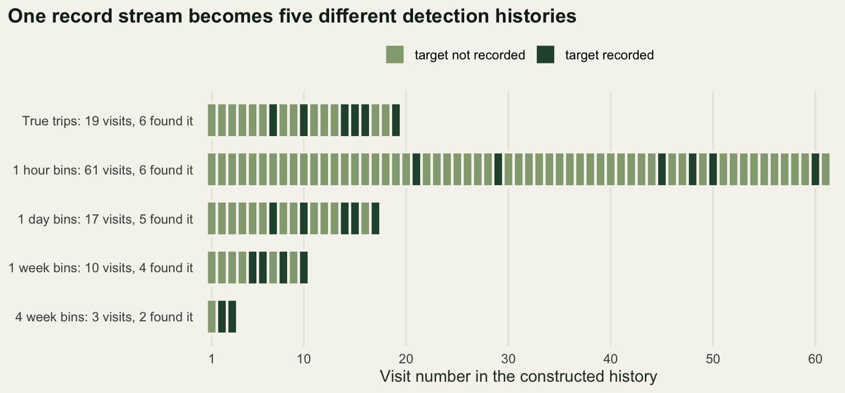
The busiest cell shows what the choice does to a single site. 19 real trips found the species six times. Cut the same records into one hour bins and the site has 61 visits, still six of them with a record: the detections are the same events, spread across more than three times as many visits and over four times as many blanks. Widen to four week bins and the site has three visits, two of which found the species. Every row is a faithful summary of the same records, and no two of them tell the model the same story.
What a window costs
Run the county through seven window widths, from one hour to four weeks, keeping the spatial unit at one kilometre and ignoring recorder identity, which is the situation when the database gives you a place and a date and nothing else. Sixty replicate seasons, each with a fresh landscape, fresh recorders and fresh detections.
n_rep <- 60
wins <- c(1, 3, 6, 24, 72, 168, 672)
win_lab <- c("1 hour", "3 hours", "6 hours", "1 day", "3 days", "1 week", "4 weeks")
print(c(replicate_seasons = n_rep, windows = length(wins)))
replicate_seasons windows
60 7 set.seed(20260804)
res_w <- array(NA_real_, c(n_rep, length(wins), 6))
for (r in seq_len(n_rep)) {
tt <- simulate_trips(); pp <- trip_p(tt); bb <- background(tt)
cc <- assemble(tt, bb, pp, tt$occ[tt$cell] > 0 & runif(tt$n_trip) < pp$p)
for (j in seq_along(wins)) {
h <- histories(cc$cell, visit_key(cc, wins[j], FALSE), cc$tgt)
fo <- fit_occ(h$K, h$Y)
res_w[r, j, ] <- c(fo[1], fo[2], mean(h$K), sum(h$K) / tt$n_trip,
mean(cc$occ[h$site]), length(h$K))
}
}
wm <- apply(res_w, c(2, 3), mean)
dimnames(wm) <- list(win_lab, c("psi", "p", "visits_per_site", "visits_per_trip",
"true_psi", "sites"))
print(round(wm, 4)) psi p visits_per_site visits_per_trip true_psi sites
1 hour 0.3421 0.1036 10.2608 3.0528 0.3022 750.7167
3 hours 0.3276 0.1939 5.7109 1.6991 0.3022 750.7167
6 hours 0.3189 0.2601 4.3693 1.3000 0.3022 750.7167
1 day 0.3034 0.3528 3.3210 0.9881 0.3022 750.7167
3 days 0.3003 0.3667 3.1673 0.9424 0.3022 750.7167
1 week 0.2960 0.3908 2.9009 0.8633 0.3022 750.7167
4 weeks 0.2861 0.4897 2.0383 0.6068 0.3022 750.7167w_bias <- apply(res_w[, , 1] - res_w[, , 5], 2, mean)
w_bse <- apply(res_w[, , 1] - res_w[, , 5], 2, sd) / sqrt(n_rep)
names(w_bias) <- names(w_bse) <- win_lab
print(round(rbind(occupancy_bias = w_bias, monte_carlo_se = w_bse), 4)) 1 hour 3 hours 6 hours 1 day 3 days 1 week 4 weeks
occupancy_bias 0.0399 0.0254 0.0167 0.0013 -0.0019 -0.0062 -0.0161
monte_carlo_se 0.0029 0.0028 0.0028 0.0026 0.0025 0.0025 0.0025print(c(same_sites_under_every_window =
all(apply(res_w[, , 6], 1, function(z) diff(range(z))) == 0)))same_sites_under_every_window
TRUE round(c(occupancy_range_across_windows = max(wm[, 1]) - min(wm[, 1]),
lowest_detection = min(wm[, 2]), highest_detection = max(wm[, 2]),
detection_ratio = max(wm[, 2]) / min(wm[, 2]),
window_with_smallest_bias_in_hours = wins[which.min(abs(w_bias))],
overstatement_at_one_hour = w_bias[["1 hour"]],
understatement_at_four_weeks = -w_bias[["4 weeks"]]), 4) occupancy_range_across_windows lowest_detection
0.0560 0.1036
highest_detection detection_ratio
0.4897 4.7251
window_with_smallest_bias_in_hours overstatement_at_one_hour
24.0000 0.0399
understatement_at_four_weeks
0.0161 The seven answers run from 0.3421 to 0.2861, a spread of 0.0560 on a truth of 0.3022, and the detection probability runs from 0.1036 to 0.4897, a factor of 4.7251. The set of sites is identical under every window, which the check confirms: a cell has records or it does not, and no width changes that. The entire spread is the definition of a visit.
The daily window is the one that comes back right, with a bias of 0.0013 against a Monte Carlo standard error of 0.0026, and that is not luck: the simulator gives each recorder at most one trip per cell per day, so the day is the true unit of search. The three day window is also within noise at -0.0019. Everything narrower is biased upward and everything wider is biased downward, and the two errors are not the same size. One hour bins overstate occupancy by 0.0399, more than twice the 0.0161 that four week bins understate it by.
qnt <- c("Estimated occupancy", "Estimated detection", "Visits per real trip")
tru <- data.frame(quantity = factor(qnt, levels = qnt),
                  y = c(mean(wm[, 5]), p_base, 1))
se_of <- function(k) apply(res_w[, , k], 2, sd) / sqrt(n_rep)
fw <- data.frame(quantity = factor(rep(qnt, each = length(wins)), levels = qnt),
                 win = factor(rep(win_lab, 3), levels = win_lab),
                 y = c(wm[, 1], wm[, 2], wm[, 4]),
                 half = 2 * c(se_of(1), se_of(2), se_of(4)))

ggplot(fw, aes(win, y, group = 1)) +
  geom_hline(data = tru, aes(yintercept = y), colour = te_pal$clay,
             linetype = "dashed", linewidth = 0.8) +
  geom_ribbon(aes(ymin = y - half, ymax = y + half), fill = te_pal$sage, alpha = 0.45) +
  geom_line(colour = te_pal$forest, linewidth = 0.9) +
  geom_point(colour = te_pal$forest, size = 2.2) +
  facet_wrap(~quantity, scales = "free_y") +
  scale_y_continuous(expand = expansion(mult = 0.13)) +
  labs(x = "Width of the window that defines a visit", y = NULL,
       title = "One record stream, seven answers about the same species",
       subtitle = "Dashed line: the truth. Bands are two Monte Carlo standard errors.") +
  theme_te() +
  theme(axis.text.x = element_text(angle = 30, hjust = 1),
        strip.text = element_text(colour = te_pal$ink, face = "bold"),
        plot.subtitle = element_text(colour = "#2c3a31", size = 9),
        plot.title.position = "plot")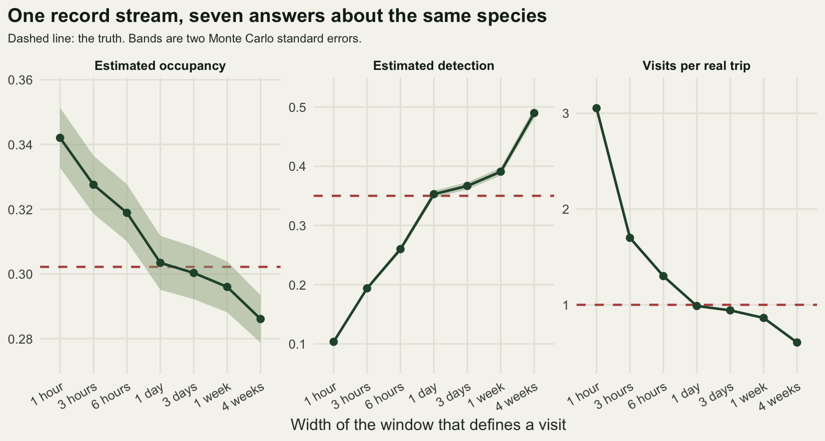
The asymmetry has an arithmetic explanation, and it is worth doing because it says which mistake to be afraid of. Splitting one trip into m visits leaves the chance of detecting the species during that trip untouched, so the model has to fit the same event with m chances instead of one. It does that by shrinking p towards p over m, and the trouble is that a site can then look blank far more easily than it should: one minus p over m, raised to the power m, is larger than one minus p for every m above one. The model therefore hands out too many blank histories to occupied sites, and compensates by raising occupancy.
Merging has no such effect. Pooling m trips into one visit raises the per-visit detection probability to one minus the m-th power of one minus p, and the chance that a site with T trips comes out blank is then exactly what it was before, because the two exponents cancel.
m1 <- wm["1 hour", "visits_per_trip"]
round(c(splits_per_trip = m1, blank_chance_truth = 1 - p_base,
        blank_chance_after_splitting = (1 - p_base / m1)^m1,
        predicted_occupancy = mean(wm[, 5]) * p_base / (1 - (1 - p_base / m1)^m1),
        measured_occupancy = wm["1 hour", "psi"]), 4)
splits_per_trip blank_chance_truth
3.0528 0.6500
blank_chance_after_splitting predicted_occupancy
0.6895 0.3407
measured_occupancy
0.3421 n_merge <- 4
merged <- (1 - (1 - (1 - p_base)^2))^(n_merge / 2)
round(c(trips = n_merge, blank_chance_truth = (1 - p_base)^n_merge,
blank_chance_after_merging = merged,
difference = (1 - p_base)^n_merge - merged), 10) trips blank_chance_truth
4.0000000 0.1785063
blank_chance_after_merging difference
0.1785063 0.0000000 kk <- visit_key(rc, 672, FALSE)
per_visit <- tapply(rc$trip, match(kk, unique(kk)), function(z) length(unique(z)))
round(c(mean_trips_per_visit = mean(per_visit), sd_trips_per_visit = sd(per_visit),
most_trips_in_one_visit = max(per_visit)), 4) mean_trips_per_visit sd_trips_per_visit most_trips_in_one_visit
1.6018 0.9547 8.0000 At the one hour window each trip becomes 3.0528 visits. A cell searched once has a 0.65 chance of coming back blank if the species is there, and the model believes that chance is 0.6895. Feed that gap through and a one visit cell should push the estimate to 0.3407; the measured value is 0.3421. The merging identity holds to every digit R prints: four trips pooled two at a time give a blank probability of 0.1785063 either way, and the difference between the two is 0.
So why is the four week window biased at all? Because merging is only harmless when it is uniform. In this season a four week visit swallows 1.6018 trips on average, with a standard deviation of 0.9547 and a worst case of 8. Visits that pool eight trips have a much higher detection probability than visits that pool one, the constant-p model splits the difference, and the leftover variation in per-visit detection comes out of occupancy. The cost of that is real but small. The cost of splitting is larger, and splitting is what you get by accident when a database timestamps records to the minute and somebody writes the obvious grouping code.
One visit per site is not an occupancy design
Widening the window has a limit. Take it to the whole season and every cell with records has exactly one visit, which is where the model stops being a model.
h_season <- histories(rc$cell, visit_key(rc, season_days * 24, FALSE), rc$tgt)
theta <- mean(h_season$Y > 0)
grid_psi <- c(0.25, 0.4, 0.6, 0.9)
ll_ridge <- sapply(grid_psi, function(z) -occ_nll(qlogis(c(z, theta / z)),
                                                  h_season$K, h_season$Y))
print(round(rbind(occupancy = grid_psi, detection = theta / grid_psi,
                  log_likelihood = ll_ridge), 6))
[,1] [,2] [,3] [,4]
occupancy 0.250000 0.400000 0.600000 0.900000
detection 0.818068 0.511292 0.340862 0.227241
log_likelihood -403.760859 -403.760859 -403.760859 -403.760859print(c(every_site_has_exactly_one_visit = all(h_season$K == 1)))every_site_has_exactly_one_visit
TRUE round(c(sites = length(h_season$K), product_of_the_two = theta,
spread_of_log_likelihood_along_the_ridge = max(ll_ridge) - min(ll_ridge)), 12) sites
797.0000000
product_of_the_two
0.2045169
spread_of_log_likelihood_along_the_ridge
0.0000000 With one visit everywhere the likelihood depends on psi and p only through their product, which the data pin at 0.2045. A county with occupancy 0.25 and detection 0.818068, and one with occupancy 0.9 and detection 0.227241, are the same claim about the records: the log likelihood is -403.760859 at both, and the spread across the four points on that ridge is 0 to twelve decimal places. optim will still return a number, and it will be whatever the starting value drifted towards.
This is the reason the sweep stops at four weeks. A season long window is not a wide window; it is the destruction of the repeat-visit structure that the whole method runs on.
The same decision on the spatial axis
A visit needs a place as well as a time. Nothing forces the analysis cell to be the one kilometre square the records were snapped to, and coarsening it is the standard response to sparse data: bigger cells collect more visits each, and the expectation is that the estimates settle down. Repeat the fit with the key on 2, 3, 4 and 6 kilometre cells, using the day and recorder grouping that was exact at the finest resolution, and compare against the truth recomputed at each cell size, where a cell counts as occupied if any of its one kilometre squares is.
grains <- c(1, 2, 3, 4, 6)
coarse_id <- function(g) ((cell_y - 1) %/% g) * (grid_x %/% g) + ((cell_x - 1) %/% g) + 1
set.seed(20260804)
res_g <- array(NA_real_, c(n_rep, length(grains), 6))
for (r in seq_len(n_rep)) {
  tt <- simulate_trips(); pp <- trip_p(tt); bb <- background(tt)
  cc <- assemble(tt, bb, pp, tt$occ[tt$cell] > 0 & runif(tt$n_trip) < pp$p)
  for (j in seq_along(grains)) {
    g <- grains[j]; ci <- coarse_id(g); site <- ci[cc$cell]
    h <- histories(site, (site * 4096 + floor(cc$time / 24)) * 128 + cc$obs, cc$tgt)
    fo <- fit_occ(h$K, h$Y)
    og <- as.vector(rowsum(cc$occ, ci) > 0)
    fr <- as.vector(rowsum(cc$occ, ci)) / (g * g)
    eff <- as.vector(rowsum(rep(1, tt$n_trip), ci[tt$cell]))
    ids <- sort(unique(ci[tt$cell]))
    occupied_share <- sum(fr[ids][og[ids]] * eff[og[ids]]) / sum(eff[og[ids]])
    res_g[r, j, ] <- c(fo[1], fo[2], mean(h$K), length(h$K), mean(og[h$site]),
                       p_base * occupied_share)
  }
}
gm <- apply(res_g, c(2, 3), mean)
dimnames(gm) <- list(paste(grains, "km"),
                     c("psi", "p", "visits_per_site", "sites", "true_psi", "p_expected"))
print(round(gm, 4))
psi p visits_per_site sites true_psi p_expected
1 km 0.3043 0.3495 3.3610 750.7167 0.3022 0.3500
2 km 0.4561 0.2283 10.1663 248.1833 0.4980 0.2111
3 km 0.5512 0.1856 20.9433 120.4500 0.6260 0.1672
4 km 0.6242 0.1626 35.8335 70.3833 0.7308 0.1432
6 km 0.7902 0.1311 79.0378 31.9000 0.8882 0.1192g_bias <- apply(res_g[, , 1] - res_g[, , 5], 2, mean)
g_bse <- apply(res_g[, , 1] - res_g[, , 5], 2, sd) / sqrt(n_rep)
names(g_bias) <- names(g_bse) <- paste(grains, "km")
print(round(rbind(occupancy_bias = g_bias, monte_carlo_se = g_bse), 4)) 1 km 2 km 3 km 4 km 6 km
occupancy_bias 0.0021 -0.0419 -0.0748 -0.1066 -0.098
monte_carlo_se 0.0026 0.0035 0.0039 0.0056 0.006round(c(worst_bias = min(g_bias), worst_bias_at_km = grains[which.min(g_bias)],
detection_at_1km_over_6km = gm[1, 2] / gm[5, 2]), 4) worst_bias worst_bias_at_km detection_at_1km_over_6km
-0.1066 4.0000 2.6658 True occupancy climbs from 0.3022 to 0.8882 as the cell side goes from 1 to 6 kilometres, which is not a finding but a definition: a block six kilometres on a side is occupied if any square kilometre inside it is. The reported quantity changes meaning under you, and the same is true of detection, which falls from 0.3495 to 0.1311, a factor of 2.6658. A visit to a 6 kilometre cell is still a three hour walk in one square kilometre of it, so the recorder now has to be in the right part of the cell as well as lucky, and p has quietly become a product of availability and detection.
That much is bookkeeping. The measurement underneath is not. The estimator tracks true occupancy exactly at 1 kilometre, with a bias of 0.0021 against a standard error of 0.0026, and then falls away from it: -0.0419 at 2 kilometres, -0.0748 at 3, and -0.1066 at 4, where the standard error is 0.0056. Coarsening the grid buys 79.0378 visits per site at 6 kilometres against 3.3610 at 1, and spends the gain on a bias that was not there at the fine resolution. The reason is in the same column: the fitted detection probability sits above the availability calculation on every coarsened grid, 0.1626 against 0.1432 at 4 kilometres, because the coarse cells differ in how much of them the species occupies, and the cells where it is everywhere dominate the detections. A constant-p model reads that spread as high detection, and any cell that came back blank then looks genuinely empty rather than under-searched.
This is the grain dependence that patch metrics and fragmentation measures on the landscape side, where patch counts and edge density move with pixel size and no single number survives a change of resolution. Occupancy behaves the same way, with the extra twist that the detection parameter absorbs part of the change.
q3 <- c("Occupancy", "Detection per visit")
f3 <- rbind(
  data.frame(km = grains, quantity = q3[1], what = "estimate", y = gm[, 1]),
  data.frame(km = grains, quantity = q3[1], what = "truth at this cell size", y = gm[, 5]),
  data.frame(km = grains, quantity = q3[2], what = "estimate", y = gm[, 2]),
  data.frame(km = grains, quantity = q3[2], what = "expected from the occupied share",
             y = gm[, 6]))
f3$quantity <- factor(f3$quantity, levels = q3)
f3$what <- factor(f3$what, levels = c("estimate", "truth at this cell size",
                                      "expected from the occupied share"))

ggplot(f3, aes(km, y, colour = what, linetype = what)) +
  geom_line(linewidth = 0.9) +
  geom_point(size = 2.4) +
  facet_wrap(~quantity, scales = "free_y") +
  scale_colour_manual(values = c("estimate" = te_pal$forest,
                                 "truth at this cell size" = te_pal$clay,
                                 "expected from the occupied share" = te_pal$gold),
                      name = NULL) +
  scale_linetype_manual(values = c("estimate" = "solid",
                                   "truth at this cell size" = "dashed",
                                   "expected from the occupied share" = "dashed"),
                        name = NULL) +
  scale_x_continuous(breaks = grains) +
  labs(x = "Side of the analysis cell (km)", y = NULL,
       title = "Bigger cells hold more of the species and less of the recorder",
       subtitle = paste("The solid estimate is drawn in both panels; each dashed",
                        "reference belongs to one panel only, so every panel has",
                        "two lines and not three.")) +
  theme_te() +
  theme(legend.position = "top",
        strip.text = element_text(colour = te_pal$ink, face = "bold"),
        plot.subtitle = element_text(colour = "#2c3a31", size = 9),
        plot.title.position = "plot")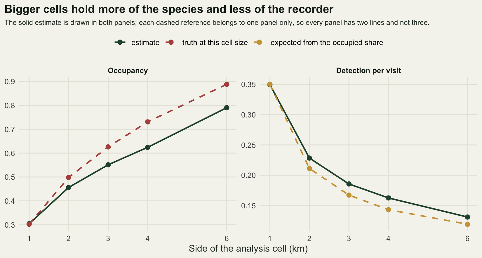
Visits by the same person are not independent visits
Everything above assumed one detection probability for everybody. Recorders differ, and in a recording scheme the good ones and the poor ones are not sprinkled evenly over the county: they each work a patch near home, so a cell tends to be searched again and again by the same person. The visits at a site are then repeats of one search rather than independent draws, and the model has no way to know.
Three versions of the same season separate the two ingredients. All three use the exact visit reconstruction, the same landscape, the same trips and the same random numbers for detection, so nothing except recorder skill differs. In the first, everybody detects at 0.35. In the second, skill varies with a standard deviation of 1.1 on the logit scale, but the skills are shuffled across trips so that a cell’s visits come from different people. In the third, the same skills stay attached to the recorders who made the trips.
n_dep <- 60
skill_sd <- 1.1
scen_lab <- c("one skill for all", "mixed skill, spread", "mixed skill, loyal")
print(c(paired_seasons = n_dep, skill_sd_on_the_logit_scale = skill_sd))
paired_seasons skill_sd_on_the_logit_scale
60.0 1.1 set.seed(20260804)
dep <- array(NA_real_, c(n_dep, 3, 6))
for (r in seq_len(n_dep)) {
tt <- simulate_trips(); bb <- background(tt); uu <- runif(tt$n_trip)
for (s in 1:3) {
pp <- switch(s, trip_p(tt), trip_p(tt, skill_sd, TRUE), trip_p(tt, skill_sd, FALSE))
cc <- assemble(tt, bb, pp, tt$occ[tt$cell] > 0 & uu < pp$p)
h <- histories(cc$cell, cc$trip, cc$tgt)
fo <- fit_occ(h$K, h$Y)
site_p <- as.vector(rowsum(pp$p, tt$cell)) /
as.vector(rowsum(rep(1, tt$n_trip), tt$cell))
dep[r, s, ] <- c(fo[1], fo[2], mean(cc$occ[h$site]), mean(pp$p),
tt$n_trip / length(unique(tt$cell * 128 + pp$obs)), sd(site_p))
}
}
dm <- apply(dep, c(2, 3), mean)
dimnames(dm) <- list(scen_lab, c("psi", "p", "true_psi", "mean_true_p",
"visits_per_recorder_cell", "sd_of_site_detection"))
print(round(dm, 4)) psi p true_psi mean_true_p visits_per_recorder_cell
one skill for all 0.3048 0.3505 0.3034 0.35 2.0913
mixed skill, spread 0.3064 0.3460 0.3034 0.35 1.0319
mixed skill, loyal 0.2768 0.3786 0.3034 0.35 2.0913
sd_of_site_detection
one skill for all 0.0000
mixed skill, spread 0.1429
mixed skill, loyal 0.1818db <- cbind(occupancy_bias = apply(dep[, , 1] - dep[, , 3], 2, mean),
se_1 = apply(dep[, , 1] - dep[, , 3], 2, sd) / sqrt(n_dep),
detection_bias = apply(dep[, , 2] - dep[, , 4], 2, mean),
se_2 = apply(dep[, , 2] - dep[, , 4], 2, sd) / sqrt(n_dep))
rownames(db) <- scen_lab
print(round(db, 4)) occupancy_bias se_1 detection_bias se_2
one skill for all 0.0015 0.0023 0.0005 0.0027
mixed skill, spread 0.0031 0.0023 -0.0040 0.0026
mixed skill, loyal -0.0265 0.0025 0.0286 0.0053round(c(share_of_occupancy_lost_when_loyal = -db[3, 1] / dm[3, 3],
share_of_detection_gained_when_loyal = db[3, 3] / dm[3, 4]), 4) share_of_occupancy_lost_when_loyal share_of_detection_gained_when_loyal
0.0874 0.0817 Skill variation on its own is harmless. With the skills shuffled across trips the occupancy bias is 0.0031 and the detection bias is -0.004, both inside two Monte Carlo standard errors of the unbiased baseline, even though the spread of site-level detection probability is 0.1429 rather than zero. Averaging within a site does the work: the same trips happen in the same places, but each cell now sees 1.0319 visits per recorder instead of 2.0913, so a poor recorder’s cell is rescued by somebody better turning up.
Let the recorders keep their own patches and the estimate breaks. Occupancy comes back at 0.2768 against a truth of 0.3034, a bias of -0.0265 with a standard error of 0.0025, and detection climbs to 0.3786, a bias of 0.0286. In relative terms the county loses 0.0874 of its occupied area and gains 0.0817 of detection probability, and the two errors are the same error: the fit sees the well-searched cells of the good recorders, concludes that detection is high, and then reads the blank histories in the poor recorders’ patches as genuine absence.
Occupancy does not survive this one, which is worth saying plainly because the hope going in was that it might. Detection is the parameter that soaks up recorder skill in every occupancy paper, and it would be convenient if psi were the sturdy one. Here the two are damaged by close to the same proportion, in opposite directions, and the damage is invisible from inside the fit: the standard errors do not widen, the estimate is simply in the wrong place. The fix is not a better window. It is a detection covariate for the recorder, which is what occupancy with detection covariates is for, and it needs the recorder identity that the window sweep above threw away.
q4 <- c("Occupancy bias", "Detection bias")
f4 <- rbind(
  data.frame(scen = rep(scen_lab, each = n_dep), quantity = q4[1],
             y = as.vector(dep[, , 1] - dep[, , 3])),
  data.frame(scen = rep(scen_lab, each = n_dep), quantity = q4[2],
             y = as.vector(dep[, , 2] - dep[, , 4])))
f4$scen <- factor(f4$scen, levels = scen_lab)
f4$quantity <- factor(f4$quantity, levels = q4)

ggplot(f4, aes(scen, y)) +
  geom_hline(yintercept = 0, colour = te_pal$clay, linetype = "dashed",
             linewidth = 0.8) +
  geom_boxplot(fill = te_pal$sage, colour = te_pal$forest, width = 0.55,
               outlier.size = 0.9, outlier.colour = te_pal$ink) +
  facet_wrap(~quantity) +
  scale_x_discrete(labels = function(z) sub(", ", ",\n", z)) +
  labs(x = NULL, y = "Estimate minus truth",
       title = "Loyal recorders break what spread-out recorders leave intact",
       subtitle = "Sixty paired seasons: same landscape, same trips, same luck.") +
  theme_te() +
  theme(strip.text = element_text(colour = te_pal$ink, face = "bold"),
        plot.subtitle = element_text(colour = "#2c3a31", size = 9),
        plot.title.position = "plot")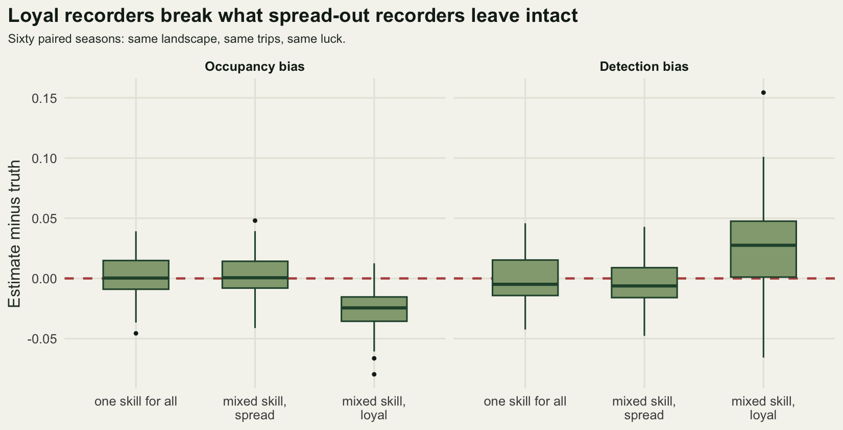
The honest limit
The deepest assumption in this post has been sitting in the simulator since the first chunk: every trip leaves at least one record behind, so every search is visible in the database. That is what makes a blank visit a blank visit rather than an absence of evidence. Recording schemes for conspicuous groups come close to it, since somebody who goes out for the morning writes down several species. Schemes where people report only the interesting find do not come close at all.
n_sil <- 40
share_seen <- 0.30
set.seed(20260804)
sil <- array(NA_real_, c(n_sil, 2, 5))
for (r in seq_len(n_sil)) {
  tt <- simulate_trips(); pp <- trip_p(tt)
  seen <- tt$occ[tt$cell] > 0 & runif(tt$n_trip) < pp$p
  for (s in 1:2) {
    bb <- if (s == 1) background(tt) else
      background(tt, share = share_seen, extra = list_rate - 1)
    cc <- assemble(tt, bb, pp, seen)
    h <- histories(cc$cell, cc$trip, cc$tgt)
    fo <- fit_occ(h$K, h$Y)
    sil[r, s, ] <- c(fo[1], fo[2], mean(cc$occ[h$site]), sum(h$K) / tt$n_trip,
                     length(h$K))
  }
}
sm <- apply(sil, c(2, 3), mean)
dimnames(sm) <- list(c("every trip leaves a record", "most trips leave nothing"),
                     c("psi", "p", "true_psi", "share_of_trips_recovered", "sites"))
print(round(sm, 4))
psi p true_psi share_of_trips_recovered
every trip leaves a record 0.2944 0.3535 0.2979 1.000
most trips leave nothing 0.3945 0.6173 0.3626 0.374
sites
every trip leaves a record 754.95
most trips leave nothing 502.00round(c(share_of_trips_reporting_anything = share_seen,
detection_inflation = sm[2, 2] / p_base,
estimate_against_the_whole_county = sm[2, 1] / psi_target), 4)share_of_trips_reporting_anything detection_inflation
0.3000 1.7638
estimate_against_the_whole_county
1.3150 Cut the reporting rate so that only 0.3 of trips mention any other species, and the visit reconstruction recovers 0.374 of the searches. The ones it recovers are not a random sample of them: a trip that found the target is always visible, because the target record is itself a record. The fitted detection probability climbs to 0.6173, 1.7638 times the truth, and occupancy comes out at 0.3945 on 502 sites whose real occupancy is 0.3626, itself well above the county figure because cells only enter the analysis if something was written down in them. Against the county’s true 0.30 the estimate is 1.315 times too high. Nothing in the output announces this; the model is perfectly happy.
Three further limits are worth naming without measuring. Effort here was clumped in space but placed without regard to the species, which is the assumption that made the visited cells a fair sample; real recorders go to nature reserves and roadsides, and that bias is a different problem with a different fix, treated in sampling bias in presence-only models. Closure within the season was exact, so a cell that was occupied in May was occupied in August, and a species that arrives or leaves mid-season will inflate detection and depress occupancy in ways the window sweep cannot separate from the effects measured here. And this was one species with a constant psi and a constant p across the county, which is the model the likelihood assumes rather than a claim about any real species.
Where to go next
The natural next step is the covariate version of everything above. Recorder identity, list length and date all belong in the detection part of the model rather than in the grouping key, and occupancy with detection covariates puts them there. List-length analysis for opportunistic data takes the other route entirely, keeping the records as records and conditioning on effort inside a regression, which avoids the visit definition problem by never constructing a visit.
If the plan is to build a trend from several seasons of records rather than one, the errors measured here compound in a way that is worth checking before anybody plots a line. Checking an unstructured-data analysis runs that set of checks, including the one this post did not: what a handful of properly designed survey sites buys when it is analysed alongside the record stream rather than instead of it.
References
MacKenzie DI, Nichols JD, Lachman GB, Droege S, Royle JA, Langtimm CA 2002 Ecology 83(8):2248-2255 (10.1890/0012-9658(2002)083[2248:ESORWD]2.0.CO;2)
Rota CT, Fletcher RJ, Dorazio RM, Betts MG 2009 Journal of Applied Ecology 46(6):1173-1181 (10.1111/j.1365-2664.2009.01734.x)
van Strien AJ, van Swaay CAM, Termaat T 2013 Journal of Applied Ecology 50(6):1450-1458 (10.1111/1365-2664.12158)
Isaac NJB, van Strien AJ, August TA, de Zeeuw MP, Roy DB 2014 Methods in Ecology and Evolution 5(10):1052-1060 (10.1111/2041-210X.12254)
Kery M, Royle JA 2016 Applied Hierarchical Modeling in Ecology, Volume 1. Academic Press, ISBN 978-0-12-801378-6