library(ggplot2)
library(patchwork)

te_paper  <- "#f5f4ee"
te_ink    <- "#16241d"
te_body   <- "#2c3a31"
te_forest <- "#275139"
te_rust   <- "#b5534e"
te_gold   <- "#c9b458"
te_line   <- "#dad9ca"

theme_datasheet <- function() {
  theme_minimal(base_size = 12) +
    theme(plot.background  = element_rect(fill = te_paper, colour = NA),
          panel.background = element_rect(fill = te_paper, colour = NA),
          panel.grid.major = element_line(colour = te_line, linewidth = 0.3),
          panel.grid.minor = element_blank(),
          text             = element_text(colour = te_body),
          plot.title       = element_text(colour = te_ink, face = "bold"),
          plot.subtitle    = element_text(colour = te_body),
          axis.text        = element_text(colour = te_body))
}Revisits triggered by sightings in occupancy data
R
occupancy
imperfect detection
citizen science
simulation
ecology tutorial
Revisits after a recorded sighting leave occupancy unbiased; revisits led by local knowledge inflate it. Tested in R, with a visit-count repair that can fail.
A scarce dragonfly turns up at a gravel pit on a Sunday morning, somebody posts the record, and by the following weekend a dozen people have been back to look. Most of them see it and log it. The same county has fifty other pits that were each checked three times in the season by whoever happened to pass. When the season’s lists are turned into detection histories, the gravel pit has fourteen visits and the others have three, and the extra visits went there because of what the data already said.
The first worry is that this breaks the occupancy model. The sites with many visits are not a random draw of sites: they were chosen after a detection. The second worry, less often voiced, is the one that should keep people awake. Many revisits are not triggered by a record at all. A warden knows the orchid is in the far meadow, a local birder knows the owl uses the barn, and they go back again and again to places they know are occupied, whether or not the first visits that season found anything. Those revisits are chosen by the true state of the site, and the true state is exactly what the model is trying to estimate.
Neither worry is new, and this post is a demonstration of known theory rather than a finding. Rubin 1976 set out when a missing-data or selection mechanism can be ignored in likelihood inference: when it depends only on quantities that were observed. Diggle, Menezes and Su 2010 showed what happens in geostatistics when sampling locations depend on the unobserved surface itself, which they called preferential sampling, and fitted a joint model for locations and values. Conn, Thorson and Johnson 2017 brought the same diagnosis to animal population distributions. What follows puts those results into single-season occupancy with numbers attached: how much a sighting-triggered rule inflates a reporting rate, whether it harms the occupancy estimate, how large the bias is when the rule reads the latent state instead, how that bias depends on detection probability, and whether a joint model of the visit counts repairs it when its own assumptions are wrong.
Three neighbours on this site set the boundaries. Adaptive cluster sampling in R is the classic data-dependent design: units are added around every find, and its section on why the naive mean is biased repairs that with design weights, because its estimator is design-based. The occupancy likelihood used here is model-based and needs no weights for a rule that reads only recorded data. Occupancy from unstructured records builds visits from a record stream and notes among its limits that effort there was “placed without regard to the species”; this post breaks exactly that assumption. What a detection time is worth costs stopping at the first detection as a design choice measured in standard error; here a detection changes the number of later visits, and the question is bias. The language of ignorable and non-ignorable mechanisms is set out for a plain regression response in missing data: MCAR, MAR and MNAR.
Three rules for sending people back
Every simulated county has 500 sites, a true occupancy of 0.25 and a per-visit detection probability of 0.25, and every site gets three base visits. On top of that, three rules decide who comes back. Under the fixed rule nobody does. Under the sighting rule, a site with at least one detection in its base visits receives a Poisson number of extra visits with mean 6. Under the latent rule, an occupied site receives the same Poisson number of extra visits with probability 0.6, whether or not anything was detected, and an empty site receives none. These constants were set before anything was run and are not tuned later.
n_site   <- 500     # sites per county
psi_true <- 0.25    # true occupancy
p_true   <- 0.25    # per-visit detection probability
k_base   <- 3       # base visits at every site
mu_extra <- 6       # mean number of extra visits when a site is revisited
a_latent <- 0.6     # latent rule: chance an occupied site draws extra visits

simulate_sites <- function(rule, n = n_site, psi = psi_true, p = p_true,
                           k0 = k_base, lam = mu_extra, a = a_latent,
                           b = 0, lam0 = lam) {
  z  <- rbinom(n, 1, psi)
  yb <- rbinom(n, k0, z * p)
  u  <- runif(n)
  e  <- switch(rule,
    fixed    = integer(n),
    sighting = ifelse(yb > 0, rpois(n, lam), 0L),
    latent   = ifelse(z == 1 & u < a, rpois(n, lam),
                      ifelse(z == 0 & u < b, rpois(n, lam0), 0L)))
  y <- yb + rbinom(n, e, z * p)
  list(y = y, e = e, z = z, yb = yb, k0 = k0)
}
The arguments b and lam0 are for later: they let empty sites draw extra visits too, the rumour that sends people to a place where the species is not. Until the last section they stay at zero.
The analysis model is the MacKenzie et al. 2002 likelihood with a different number of visits at each site. A site with y detections in K visits contributes psi p^y (1 - p)^(K - y), plus 1 - psi when y is zero. Sites that share the same detections and the same number of extra visits contribute identical terms, so the data are collapsed to those unique rows with a count, which makes each fit a few milliseconds.
collapse_sites <- function(y, e) {
  key <- y * 1000L + e
  tb  <- tabulate(key + 1L)
  k   <- which(tb > 0) - 1L
  list(y = k %/% 1000L, e = k %% 1000L, w = tb[k + 1L])
}

nll_cond <- function(th, d, k0) {
  psi <- plogis(th[1]); p <- plogis(th[2]); K <- k0 + d$e
  -sum(d$w * log(psi * p^d$y * (1 - p)^(K - d$y) + (1 - psi) * (d$y == 0)))
}

# visit count modelled too: zero-inflated Poisson at occupied sites, none at empty sites
nll_joint <- function(th, d, k0) {
  psi <- plogis(th[1]); p <- plogis(th[2]); a1 <- plogis(th[3]); lam <- exp(th[4])
  K <- k0 + d$e
  pe1 <- a1 * dpois(d$e, lam) + (1 - a1) * (d$e == 0)
  -sum(d$w * log(psi * pe1 * p^d$y * (1 - p)^(K - d$y) +
                 (1 - psi) * (d$e == 0) * (d$y == 0)))
}

# as above, but empty sites may also draw extra visits, with their own probability
nll_flex <- function(th, d, k0) {
  psi <- plogis(th[1]); p <- plogis(th[2]); a1 <- plogis(th[3]); a0 <- plogis(th[4])
  lam <- exp(th[5]); K <- k0 + d$e
  pe1 <- a1 * dpois(d$e, lam) + (1 - a1) * (d$e == 0)
  pe0 <- a0 * dpois(d$e, lam) + (1 - a0) * (d$e == 0)
  -sum(d$w * log(psi * pe1 * p^d$y * (1 - p)^(K - d$y) + (1 - psi) * pe0 * (d$y == 0)))
}

nll_of   <- list(cond = nll_cond, joint = nll_joint, flex = nll_flex)
start_of <- list(cond = c(0, 0), joint = c(0, 0, 0, log(4)), flex = c(0, 0, 0, -1, log(4)))

fit_occ <- function(d, k0, model = "cond", ci = FALSE) {
  o <- optim(start_of[[model]], nll_of[[model]], d = d, k0 = k0, method = "BFGS")
  out <- c(psi = plogis(o$par[1]), p = plogis(o$par[2]))
  if (ci) {
    se_logit <- sqrt(solve(optimHess(o$par, nll_of[[model]], d = d, k0 = k0))[1, 1])
    out <- c(out, lo = plogis(o$par[1] - 1.96 * se_logit),
                  hi = plogis(o$par[1] + 1.96 * se_logit))
  }
  out
}
One county under the sighting rule shows the pieces. The reporting rate is detections over all visits, and an intercept-only logistic regression on the visits, the list-based analysis that treats each visit as a trial, returns the same number.
set.seed(1709)
ex <- simulate_sites("sighting")
ex_d <- collapse_sites(ex$y, ex$e)
ex_fit <- fit_occ(ex_d, ex$k0, ci = TRUE)
ex_rr <- sum(ex$y) / sum(ex$k0 + ex$e)
ex_glm <- glm(cbind(ex$y, ex$k0 + ex$e - ex$y) ~ 1, family = binomial)
ex_glm_gap <- abs(plogis(coef(ex_glm)[[1]]) - ex_rr)
ex_revisited <- sum(ex$e > 0); ex_rows <- length(ex_d$w)
ex_true_occ <- mean(ex$z)
round(c(ex_fit, rr = ex_rr), 3)
psi p lo hi rr
0.306 0.218 0.240 0.381 0.104 In this county 80 sites were revisited, and the 500 sites collapse to 35 distinct rows. The occupancy estimate is 0.306 with a 95 per cent interval from 0.240 to 0.381, against a realised share of occupied sites of 0.252, and detection comes out at 0.218. The reporting rate is 0.104, and the logistic regression reproduces it to 2.4e-10. One county proves nothing; the next section repeats it.
A rule that reads the records is ignorable
set.seed(4101)
n_rep_main <- 400   # fixed before any estimate was inspected
rules <- c("fixed", "sighting", "latent")
main <- do.call(rbind, lapply(seq_len(n_rep_main), function(r)
  do.call(rbind, lapply(rules, function(rl) {
    s <- simulate_sites(rl)
    d <- collapse_sites(s$y, s$e)
    f <- fit_occ(d, s$k0, ci = TRUE)
    jj <- if (rl == "latent") fit_occ(d, s$k0, "joint")[["psi"]] else NA_real_
    data.frame(rep = r, rule = rl, rr = sum(s$y) / sum(s$k0 + s$e),
               naive = mean(s$y > 0), psi = f[["psi"]], p = f[["p"]],
               cover = f[["lo"]] <= psi_true & f[["hi"]] >= psi_true, joint = jj,
               det_rev = if (any(s$e > 0)) mean(s$y[s$e > 0] > 0) else NA_real_,
               # fit check at revisited sites: observed and model-implied share with no detection
               zero_obs = if (any(s$e > 0)) mean(s$y[s$e > 0] == 0) else NA_real_,
               zero_fit = if (any(s$e > 0)) mean(1 - f[["psi"]] + f[["psi"]] *
                            (1 - f[["p"]])^(s$k0 + s$e[s$e > 0])) else NA_real_,
               # timing: revisited sites with nothing recorded before the extra visits began
               base_none = if (any(s$e > 0)) mean(s$yb[s$e > 0] == 0) else NA_real_)
  }))))
by_rule <- function(col, fun = mean) vapply(rules, function(rl) fun(main[main$rule == rl, col]), 0)
m_psi <- by_rule("psi"); s_psi <- by_rule("psi", sd); m_p <- by_rule("p")
m_rr <- by_rule("rr"); m_naive <- by_rule("naive"); m_cover <- by_rule("cover")
m_joint <- mean(main$joint[main$rule == "latent"])
det_rev_latent <- mean(main$det_rev[main$rule == "latent"])
s_joint <- sd(main$joint[main$rule == "latent"])
mcse_psi <- s_psi / sqrt(n_rep_main)
mcse_cover <- sqrt(0.95 * 0.05 / n_rep_main)

rr_closed <- function(rule, psi = psi_true, p = p_true, k0 = k_base,
                      lam = mu_extra, a = a_latent) {
  q <- if (rule == "sighting") 1 - (1 - p)^k0 else a
  psi * p * (k0 + q * lam) / (k0 + psi * q * lam)
}
rr_arith <- c(fixed = psi_true * p_true, sighting = rr_closed("sighting"),
              latent = rr_closed("latent"))
infl_sight <- m_rr[["sighting"]] / m_rr[["fixed"]]
bias_latent <- 100 * (m_psi[["latent"]] / psi_true - 1)
sd_ratio <- s_psi[["sighting"]] / s_psi[["fixed"]]
round(rbind(psi = m_psi, sd = s_psi, p = m_p, rr = m_rr, naive = m_naive, cover = m_cover), 3)
fixed sighting latent
psi 0.258 0.250 0.383
sd 0.048 0.031 0.047
p 0.249 0.249 0.207
rr 0.062 0.103 0.105
naive 0.144 0.143 0.193
cover 0.953 0.953 0.092Over 400 counties the fixed design estimates occupancy at 0.258 with a spread of 0.048 between counties. The sighting rule, applied to counties drawn the same way, estimates 0.250 with a spread of 0.031, 0.65 times the fixed design’s. The Monte Carlo standard errors of the two means are 0.0024 and 0.0015. The sighting rule shows no bias these runs can detect. The fixed design sits 3.2 standard errors above the truth, a small-sample bias of a three-visit design at low detection; the triggered visits at a mean of six extra visits shrink it below what these runs can detect, and the grid below leaves a possible trace at a mean of two. The triggered design is also the more precise of the two, because it spends its extra visits where detection information is worth having. The Wald intervals cover the true 0.25 in 95.2 and 95.2 per cent of counties, with a Monte Carlo standard error of 1.1 points.
That is Rubin’s result working. The extra visits depend on the base detections, which are in the data, so the probability of the visit pattern factors out of the likelihood and carries no information about occupancy or detection. MacKenzie and Royle 2005 lean on the same fact in the other direction when they discuss a removal design, in which a site stops being visited after its first detection: the likelihood needs no correction for the number of visits being decided by the data. Rubin’s condition covers likelihood inference, and the Wald intervals here use the observed information from the fitted surface, which is the version that stays valid when the design reads the data.
The reporting rate is a different story. It rises from 0.062 to 0.103, a factor of 1.65, with no change in the species. This part needs no simulation. At an occupied site the base visits find the species with probability one minus (1 - p)^3; the expected number of detections and the expected number of visits then follow directly, and the ratio of the two expectations is 0.105, against the simulated 0.103. The naive share of sites with a detection does not move at all, 0.144 against 0.143, because the rule only sends people to sites that already had one.
The latent rule looks similar in the reporting rate, 0.105, and is nothing like it in the model. Occupancy comes out at 0.383, +53 per cent, detection falls to 0.207, and the interval covers the truth in 9.2 per cent of counties. Nothing in the estimates announces the difference.
trig <- c("sighting", "latent")
m_zero_obs <- by_rule("zero_obs")[trig]; m_zero_fit <- by_rule("zero_fit")[trig]
m_base_none <- by_rule("base_none")[trig]
base_none_arith <- (1 - p_true)^k_base
round(rbind(zero_obs = m_zero_obs, zero_fit = m_zero_fit, base_none = m_base_none), 3)
sighting latent
zero_obs 0.000 0.094
zero_fit 0.774 0.674
base_none 0.000 0.422A goodness-of-fit check does notice something, but under both rules. At revisited sites the fitted model expects a share of 0.774 with no detection under the sighting rule, and the data have 0.000; under the latent rule it expects 0.674 and the data have 0.094. A check of detections against visit counts fails under the harmless rule as well, so it cannot separate the two. What does separate them is timing. Under the sighting rule no revisited site had an empty record before its extra visits began, by construction: the share is 0.000. Under the latent rule the share is 0.422, against the (1 - p)^3 = 0.422 of occupied sites that three base visits miss.
rule_lab <- c(fixed = "no revisits", sighting = "revisit after a sighting",
              latent = "revisit occupied sites")
main$rule_f <- factor(unname(rule_lab[main$rule]), levels = rule_lab)
rule_col <- setNames(c(te_gold, te_forest, te_rust), rule_lab)
x_lab <- c("no\nrevisits", "revisit after\na sighting", "revisit\noccupied sites")

p_psi <- ggplot(main, aes(rule_f, psi, fill = rule_f)) +
  geom_hline(yintercept = psi_true, colour = te_ink, linetype = "dashed", linewidth = 0.6) +
  geom_boxplot(width = 0.55, colour = te_body, outlier.size = 0.8, linewidth = 0.4) +
  scale_fill_manual(values = rule_col, guide = "none") +
  scale_x_discrete(labels = x_lab) +
  labs(x = NULL, y = "estimated occupancy", title = "The likelihood",
       subtitle = "dashed line: true occupancy") +
  theme_datasheet()

rr_tab <- data.frame(rule_f = factor(unname(rule_lab), levels = rule_lab),
                     sim = unname(m_rr), arith = unname(rr_arith))
p_rr <- ggplot(main, aes(rule_f, rr, fill = rule_f)) +
  geom_boxplot(width = 0.55, colour = te_body, outlier.size = 0.8, linewidth = 0.4) +
  geom_point(data = rr_tab, aes(rule_f, arith), inherit.aes = FALSE,
             shape = 23, size = 3, fill = te_paper, colour = te_ink) +
  scale_fill_manual(values = rule_col, guide = "none") +
  scale_x_discrete(labels = x_lab) +
  labs(x = NULL, y = "detections per visit", title = "The reporting rate",
       subtitle = "diamonds: ratio of expectations") +
  theme_datasheet()

p_psi + p_rr + plot_annotation(theme = theme_datasheet())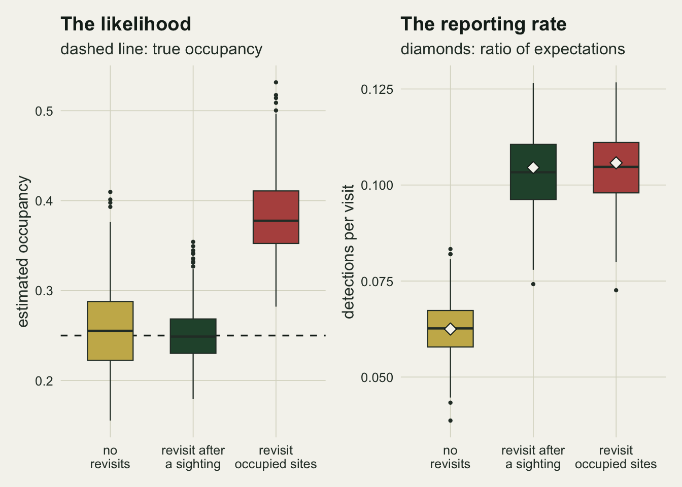
Stronger triggers, same split
The number of extra visits is the dial that alert systems turn. Raising its mean from zero to eight shows whether the two rules part company gradually.
set.seed(4102)
n_rep_grid <- 120   # per cell; fixed before any cell was inspected
lam_grid <- c(0, 2, 4, 6, 8)
grid_lam <- do.call(rbind, lapply(lam_grid, function(lm)
  do.call(rbind, lapply(c("sighting", "latent"), function(rl) {
    v <- t(replicate(n_rep_grid, {
      s <- simulate_sites(rl, lam = lm)
      c(rr = sum(s$y) / sum(s$k0 + s$e), fit_occ(collapse_sites(s$y, s$e), s$k0))
    }))
    data.frame(lam = lm, rule = rl, rr = mean(v[, "rr"]), psi = mean(v[, "psi"]),
               psi_sd = sd(v[, "psi"]))
  }))))
gl <- function(lm, rl, col) grid_lam[grid_lam$lam == lm & grid_lam$rule == rl, col]
sight_pos <- grid_lam$rule == "sighting" & grid_lam$lam > 0
sight_dev <- max(abs(grid_lam$psi[sight_pos] - psi_true))
sight_dev_lam <- grid_lam$lam[sight_pos][which.max(abs(grid_lam$psi[sight_pos] - psi_true))]
sight_mcse <- max(grid_lam$psi_sd[sight_pos]) / sqrt(n_rep_grid)
rr_gap <- max(abs(grid_lam$rr - mapply(function(lm, rl) rr_closed(rl, lam = lm),
                                       grid_lam$lam, grid_lam$rule)))
print(grid_lam, digits = 3)
lam rule rr psi psi_sd
1 0 sighting 0.0632 0.258 0.0461
2 0 latent 0.0621 0.254 0.0472
3 2 sighting 0.0793 0.257 0.0335
4 2 latent 0.0799 0.328 0.0454
5 4 sighting 0.0932 0.253 0.0313
6 4 latent 0.0938 0.360 0.0476
7 6 sighting 0.1061 0.254 0.0319
8 6 latent 0.1058 0.385 0.0481
9 8 sighting 0.1145 0.254 0.0283
10 8 latent 0.1154 0.397 0.0371With any extra visits at all, the sighting rule’s mean estimate stays within 0.007 of 0.25, against a largest Monte Carlo standard error of 0.0031 per cell, and the largest gap is at the weakest trigger, a mean of 2 extra visits; the cell with no extra visits is the fixed design again, at 0.258. The latent rule climbs from 0.328 at a mean of two extra visits to 0.397 at eight. The reporting rates of the two rules move almost together, 0.1145 and 0.1154 at eight extra visits, and the ratio-of-expectations arithmetic matches every simulated cell to 0.002. A reporting rate cannot tell the harmless trigger from the harmful one, and it is inflated by both.
grid_lam$rule_f <- factor(unname(rule_lab[grid_lam$rule]), levels = rule_lab[2:3])
lam_fine <- seq(0, 8, by = 0.1)
arith_line <- do.call(rbind, lapply(c("sighting", "latent"), function(rl)
  data.frame(lam = lam_fine, rr = vapply(lam_fine, function(lm) rr_closed(rl, lam = lm), 0),
             rule_f = factor(unname(rule_lab[rl]), levels = rule_lab[2:3]))))

p_rr_lam <- ggplot(grid_lam, aes(lam, rr, colour = rule_f)) +
  geom_line(data = arith_line, linewidth = 0.8) +
  geom_point(size = 2.4) +
  scale_colour_manual(values = rule_col[2:3], name = NULL) +
  labs(x = "mean extra visits", y = "detections per visit", title = "Reporting rate",
       subtitle = "lines: arithmetic, points: simulation") +
  theme_datasheet() + theme(legend.position = "bottom")

p_psi_lam <- ggplot(grid_lam, aes(lam, psi, colour = rule_f)) +
  geom_hline(yintercept = psi_true, colour = te_ink, linetype = "dashed", linewidth = 0.6) +
  geom_errorbar(aes(ymin = psi - 2 * psi_sd / sqrt(n_rep_grid),
                    ymax = psi + 2 * psi_sd / sqrt(n_rep_grid)), width = 0.25, linewidth = 0.5,
                show.legend = FALSE) +
  geom_line(linewidth = 0.8) + geom_point(size = 2.4) +
  scale_colour_manual(values = rule_col[2:3], name = NULL) +
  scale_y_continuous(limits = c(0.2, NA)) +
  labs(x = "mean extra visits", y = "mean estimated occupancy", title = "Occupancy likelihood",
       subtitle = "dashed: truth; bars: two MC SE") +
  theme_datasheet() + theme(legend.position = "bottom")

(p_rr_lam + p_psi_lam) + plot_layout(guides = "collect") +
  plot_annotation(theme = theme_datasheet()) & theme(legend.position = "bottom")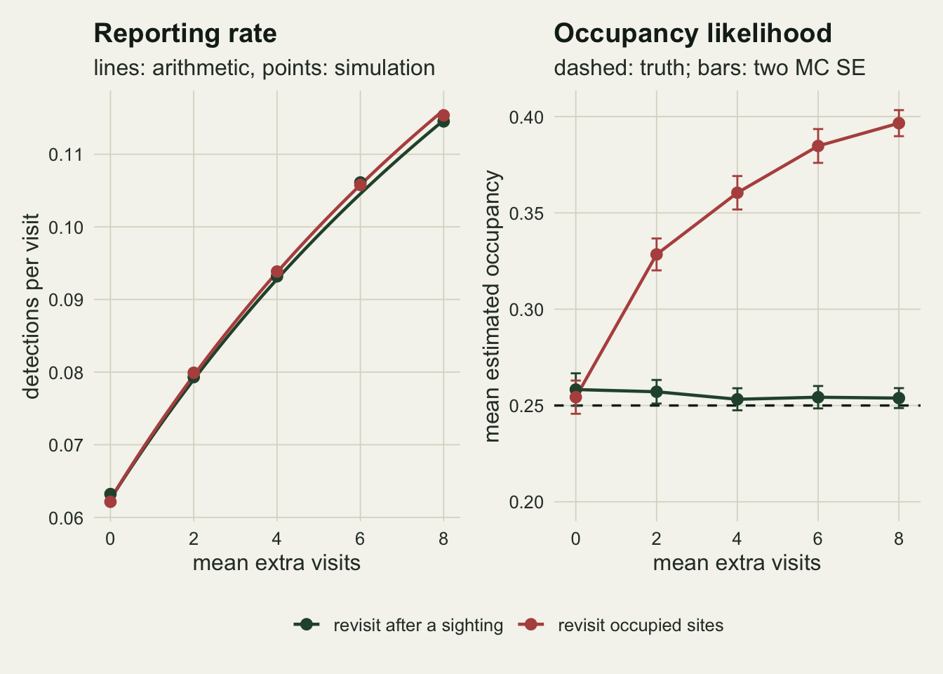
A rule that reads what nobody wrote down
The latent bias has a simple source. A site revisited under the latent rule is occupied, and with its extra visits it is usually detected: in the main comparison 90.6 per cent of revisited sites had at least one detection, so the sites with long visit records are mostly detections. The model assumes one occupancy probability for every site whatever its number of visits, so it pulls occupancy up to fit those sites and pulls detection down to explain the three-visit sites that found nothing. How much damage that does depends on how many occupied sites the base visits miss, which is (1 - p)^3 of them, and that shrinks fast as detection rises. The grid below crosses four detection probabilities with the two strengths of latent preference named in the design, 0.2 and 0.6, and fits the joint model next to the conditional one.
set.seed(4103)
p_grid <- c(0.15, 0.25, 0.3, 0.5)
a_grid <- c(0.2, 0.6)
grid_p <- do.call(rbind, lapply(p_grid, function(pp) do.call(rbind, lapply(a_grid, function(aa) {
  v <- t(replicate(n_rep_grid, {
    s <- simulate_sites("latent", p = pp, a = aa)
    d <- collapse_sites(s$y, s$e)
    c(cond = fit_occ(d, s$k0)[["psi"]], joint = fit_occ(d, s$k0, "joint")[["psi"]])
  }))
  data.frame(p = pp, a = aa, cond = mean(v[, "cond"]), joint = mean(v[, "joint"]),
             cond_sd = sd(v[, "cond"]), joint_sd = sd(v[, "joint"]))
}))))
gp <- function(pp, aa, col) grid_p[grid_p$p == pp & grid_p$a == aa, col]
bias_pct <- function(x) 100 * (x / psi_true - 1)
miss_base <- (1 - p_grid)^k_base
joint_dev <- max(abs(grid_p$joint - psi_true))
joint_mcse <- max(grid_p$joint_sd) / sqrt(n_rep_grid)
round(grid_p, 3)
p a cond joint cond_sd joint_sd
1 0.15 0.2 0.365 0.257 0.095 0.043
2 0.15 0.6 0.480 0.253 0.070 0.029
3 0.25 0.2 0.311 0.251 0.040 0.026
4 0.25 0.6 0.382 0.251 0.043 0.023
5 0.30 0.2 0.289 0.248 0.039 0.030
6 0.30 0.6 0.350 0.251 0.034 0.023
7 0.50 0.2 0.262 0.252 0.022 0.020
8 0.50 0.6 0.278 0.252 0.024 0.021At a detection probability of 0.25 the conditional likelihood overestimates occupancy by 24 per cent when occupied sites draw extra visits with probability 0.2, and by 53 per cent at 0.6. At 0.15 the two figures are 46 and 92 per cent; at 0.5 they fall to 5 and 11 per cent. The share of occupied sites that three base visits miss goes from 0.614 at the lowest detection probability to 0.125 at the highest, and the bias follows it down. The species for which this matters most is the one people revisit most: hard to find, and known to locals.
The joint model treats the number of extra visits as data with its own distribution given the state: zero-inflated Poisson at occupied sites, zero at empty sites. It is the generating model here, and it recovers occupancy in every cell, never further than 0.007 from the truth against a largest Monte Carlo standard error of 0.0039. That is the Diggle et al. 2010 recipe carried over from locations to visit counts: when the sampling depends on the latent state, model the sampling.
pg_long <- rbind(
  data.frame(p = grid_p$p, a = grid_p$a, model = "conditional likelihood",
             bias = bias_pct(grid_p$cond), se = 100 * grid_p$cond_sd / psi_true / sqrt(n_rep_grid)),
  data.frame(p = grid_p$p, a = grid_p$a, model = "joint visit-count model",
             bias = bias_pct(grid_p$joint), se = 100 * grid_p$joint_sd / psi_true / sqrt(n_rep_grid)))
pg_long$pref <- factor(sprintf("occupied sites revisited with prob. %.1f", pg_long$a))
pg_long$model <- factor(pg_long$model, levels = c("conditional likelihood", "joint visit-count model"))

ggplot(pg_long, aes(p, bias, colour = model, linetype = pref)) +
  geom_hline(yintercept = 0, colour = te_ink, linewidth = 0.5) +
  geom_errorbar(aes(ymin = bias - 2 * se, ymax = bias + 2 * se), width = 0.012,
                linewidth = 0.4, linetype = "solid") +
  geom_line(linewidth = 0.9) + geom_point(size = 2.4) +
  scale_colour_manual(values = c(te_rust, te_forest), name = NULL) +
  scale_linetype_manual(values = c("dashed", "solid"), name = NULL) +
  scale_x_continuous(breaks = p_grid) +
  guides(colour = guide_legend(nrow = 2), linetype = guide_legend(nrow = 2)) +
  labs(x = "per-visit detection probability", y = "bias in occupancy, per cent of truth",
       title = "The latent bias shrinks as detection rises",
       subtitle = "true occupancy 0.25, three base visits, bars: two Monte Carlo SE") +
  theme_datasheet() +
  theme(legend.position = "bottom", legend.key.width = grid::unit(2.2, "lines"))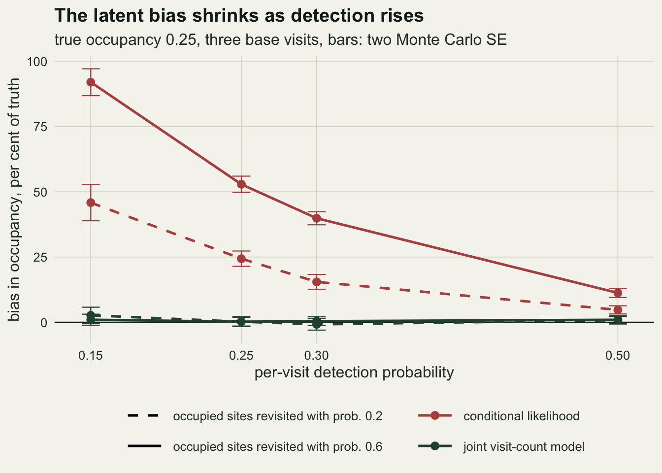
The repair rests on empty sites staying empty
The joint model above has an assumption that does a great deal of work: an empty site never draws an extra visit. Any site with an extra visit is then known to be occupied, and the model reads that off the visit count directly. Real revisits are not so tidy. A rumour sends people to a pit where the dragonfly never was, and an old record keeps a meadow on the round long after the orchid has gone. The next grid lets empty sites draw extra visits too, with probability b from 0 up to 0.6, the value at which occupied and empty sites are treated alike and the rule stops depending on the state at all. Three models are fitted to each county: the conditional likelihood, the joint model that assumes empty sites stay empty, and a flexible joint model that gives empty sites their own probability of extra visits. Two further cells stress the flexible model: rumour visits at empty sites with a smaller mean of 2 while the model assumes one mean for both states, and the ordinary rumour arm at a detection probability of 0.15.
set.seed(4104)
b_grid <- c(0, 0.1, 0.2, 0.4, 0.6)
cells <- rbind(data.frame(b = b_grid, p = p_true, lam0 = mu_extra, arm = "grid"),
               data.frame(b = 0.2, p = c(p_true, 0.15), lam0 = c(2, mu_extra),
                          arm = c("smaller rumour mean", "low detection")))
grid_b <- do.call(rbind, lapply(seq_len(nrow(cells)), function(i) {
  cc <- cells[i, ]
  v <- t(replicate(n_rep_grid, {
    s <- simulate_sites("latent", p = cc$p, b = cc$b, lam0 = cc$lam0)
    d <- collapse_sites(s$y, s$e)
    c(cond = fit_occ(d, s$k0)[["psi"]], joint = fit_occ(d, s$k0, "joint")[["psi"]],
      flex = fit_occ(d, s$k0, "flex")[["psi"]])
  }))
  data.frame(cc, cond = mean(v[, "cond"]), joint = mean(v[, "joint"]), flex = mean(v[, "flex"]),
             cond_sd = sd(v[, "cond"]), joint_sd = sd(v[, "joint"]), flex_sd = sd(v[, "flex"]))
}))
gb <- function(bb, col, arm = "grid") grid_b[grid_b$b == bb & grid_b$arm == arm, col]
flex_dev <- max(abs(grid_b$flex[grid_b$arm == "grid"] - psi_true))
flex_mcse <- max(grid_b$flex_sd[grid_b$arm == "grid"]) / sqrt(n_rep_grid)
round(grid_b[, -4], 3)
b p lam0 cond joint flex cond_sd joint_sd flex_sd
1 0.0 0.25 6 0.375 0.246 0.245 0.042 0.024 0.022
2 0.1 0.25 6 0.349 0.363 0.254 0.037 0.032 0.025
3 0.2 0.25 6 0.316 0.477 0.253 0.038 0.040 0.039
4 0.4 0.25 6 0.274 0.694 0.247 0.025 0.056 0.023
5 0.6 0.25 6 0.252 0.914 0.253 0.027 0.054 0.027
6 0.2 0.25 2 0.353 0.416 0.287 0.039 0.031 0.030
7 0.2 0.15 6 0.355 0.485 0.261 0.049 0.045 0.057A small leak is enough to break the joint model. With one empty site in ten drawing extra visits it estimates occupancy at 0.363, already worse than the conditional likelihood’s 0.349, and at b of 0.2 it gives 0.477 against 0.316. At 0.6, where the revisit rule no longer depends on the state and the conditional likelihood is back to 0.252, the joint model reports 0.914: it has declared almost every revisited site occupied. The mechanism is the same assumption that made the repair work. If an extra visit implies occupancy, every rumour visit to an empty site is counted as an occupied site where the species was missed, and detection is pulled down to explain why.
The flexible model, which lets empty sites have their own chance of extra visits, stays within 0.005 of the truth across the whole grid, with a largest Monte Carlo standard error of 0.0036. In that grid it is, like the first joint model before it, the model that generated the data: empty sites draw their visits from the same Poisson mean it assumes. It is identified because the detections separate the two states: the visit counts at sites that recorded the species describe occupied sites, and the model can learn how often the rest were revisited. That separation is also where it weakens. When rumour visits at empty sites come with a smaller mean than visits to occupied sites and the model assumes a single mean, the flexible model gives 0.287, +15 per cent (the conditional likelihood gives 0.353); this is the only cell in which the flexible model is itself wrong. At a detection probability of 0.15 it gives 0.261 against the conditional likelihood’s 0.355, but with a spread between counties of 0.057 against 0.049: less bias, bought with noise. So the answer to the obvious question is that the repair is not free. It is identified by the count model being right about empty sites. The flexible model was still the least biased of the three in both stress cells, but the joint model that assumed empty sites stay empty did more harm than no model of the visits at all from the first leak onwards.
rb <- grid_b[grid_b$arm == "grid", ]
rb_long <- data.frame(
  b = rep(rb$b, 3),
  model = factor(rep(c("conditional likelihood", "joint: empty sites stay empty",
                       "joint: empty sites revisited too"), each = nrow(rb)),
                 levels = c("conditional likelihood", "joint: empty sites stay empty",
                            "joint: empty sites revisited too")),
  psi = c(rb$cond, rb$joint, rb$flex),
  se = c(rb$cond_sd, rb$joint_sd, rb$flex_sd) / sqrt(n_rep_grid))

ggplot(rb_long, aes(b, psi, colour = model)) +
  geom_hline(yintercept = psi_true, colour = te_ink, linetype = "dashed", linewidth = 0.6) +
  geom_errorbar(aes(ymin = psi - 2 * se, ymax = psi + 2 * se), width = 0.012, linewidth = 0.4) +
  geom_line(linewidth = 0.9) + geom_point(size = 2.4) +
  scale_colour_manual(values = c(te_gold, te_rust, te_forest), name = NULL) +
  scale_x_continuous(breaks = b_grid) +
  scale_y_continuous(limits = c(0, 1)) +
  guides(colour = guide_legend(nrow = 3)) +
  labs(x = "probability an empty site draws extra visits",
       y = "mean estimated occupancy",
       title = "A visit model that is wrong about empty sites",
       subtitle = "dashed line: true occupancy; at 0.6 the rule ignores the state") +
  theme_datasheet() + theme(legend.position = "bottom")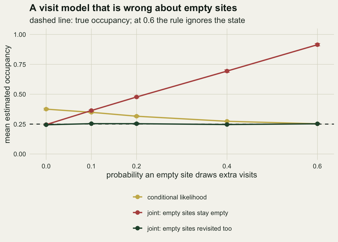
What to report
Say how visits were generated, in words, before any estimate. A fixed schedule, visits added after records, and visits by people who know the site are three different sampling mechanisms, and only the first two leave the occupancy likelihood alone.
Do not report a reporting rate, or a list-based logistic regression with no site structure, from data with triggered revisits as if it measured the species. Under the sighting rule it rose by a factor of 1.65 with occupancy unchanged. If a reporting rate must be shown, show it next to the visit counts per site, and use the arithmetic above to say how much of it the trigger could produce.
If the revisits followed recorded sightings, the conditional occupancy likelihood with each site’s own number of visits is the right analysis, with no weights and no correction, and it is worth saying that the triggered visits made the estimate more precise.
If some revisits may follow local knowledge, the data rarely say so. A record or checklist rarely stores why the visit took place; an alert source, a flag for a twitch, or a link between checklists shared by a group can sometimes be reconstructed from comments or timing, and where it can, visits that followed a public record can be separated from repeat visits by the same people to the same site. A lack of fit between visit counts and detections is not the symptom, because the harmless trigger produced it too. Where visit dates are kept, timing is: under a rule that follows records at the site, no site gets its burst of extra visits before anything was recorded there, while under a rule that follows local knowledge 42 per cent of revisited sites had recorded nothing first in these runs, at a detection probability of 0.25. A record elsewhere, at a neighbouring pit or on a county list, can also send people to a site with an empty record, so a nonzero share points to a trigger that did not read this site’s data rather than proving local knowledge. When local knowledge cannot be ruled out, report the conditional estimate together with a joint model of the visit counts that allows empty sites to be revisited, and whose rumour visits may have their own mean (a version not tested here), and treat a large gap between them as evidence of preferential revisits rather than as a choice of answer.
Honest limits
Everything here is a single season with constant occupancy and constant detection. Real triggers act through covariates and through unmeasured habitat quality: a reserve is both better habitat and more visited. Conn et al. 2017 fit that as a joint model in which sampling effort and density share a correlated spatial effect. None of that was simulated.
The latent rule is deliberately crude. People who know a site is occupied do not decide once per season with a fixed probability; they return more often at better sites, keep returning after a good day, and stop when a site goes quiet. Some of that reads recorded data and some reads memory, and a real mechanism is a mixture of the two rules measured separately here. The bias from a mixture was not measured.
The joint models share one Poisson mean for extra visits across states, and the flexible model’s failure under a smaller rumour mean shows how much rests on that. Giving each state its own mean is a small change to the code; whether it stays identified with realistic sample sizes and low detection is a question these runs did not ask. Nor did they ask what happens when the visit counts are overdispersed beyond the zero-inflated Poisson.
Two arms named in planning were left out: a false trend in reporting rates as alert use grows over the years at constant occupancy, which follows from the same arithmetic, and year-listing, where observers log a species only at their first sighting of the year, which is a removal design in disguise. Both deserve their own measurement.
The Monte Carlo runs use 400 counties for the main comparison and 120 per cell in the grids. That resolves the biases reported above, which are far larger than their standard errors, but not differences of a few thousandths between models that are both close to the truth.
References
Rubin DB 1976 Biometrika 63(3):581-592 (10.1093/biomet/63.3.581)
Diggle PJ, Menezes R, Su T-L 2010 Journal of the Royal Statistical Society Series C 59(2):191-232 (10.1111/j.1467-9876.2009.00701.x)
Conn PB, Thorson JT, Johnson DS 2017 Methods in Ecology and Evolution 8(11):1535-1546 (10.1111/2041-210X.12803)
MacKenzie DI, Nichols JD, Lachman GB, Droege S, Royle JA, Langtimm CA 2002 Ecology 83(8):2248-2255 (10.1890/0012-9658(2002)083[2248:ESORWD]2.0.CO;2)
MacKenzie DI, Royle JA 2005 Journal of Applied Ecology 42(6):1105-1114 (10.1111/j.1365-2664.2005.01098.x)