Adaptive cluster sampling in R

Build adaptive cluster sampling from scratch in R for rare, clustered species: networks, edge units, why the naive mean is biased, and the Hansen-Hurwitz fix.

Rare, clustered species are the hardest thing a fixed design has to cope with. Most quadrats hold nothing, a handful hold almost everything, and a simple random sample of a few dozen units mostly counts zeros. Adaptive cluster sampling turns that structure into an advantage: when a selected unit contains the species, you sample its neighbours too, and keep expanding as long as you keep finding it. The sample follows the organism.

The catch is that the mechanism which makes it efficient also breaks the obvious estimator. If you only expand where you find animals, the units you end up observing over-represent the dense patches, so the plain average of everything you sampled runs high. This post builds the design from scratch on a synthetic grid, shows exactly how biased the naive mean is, and derives the Hansen-Hurwitz estimator that puts it right.

A population built to defeat a fixed design

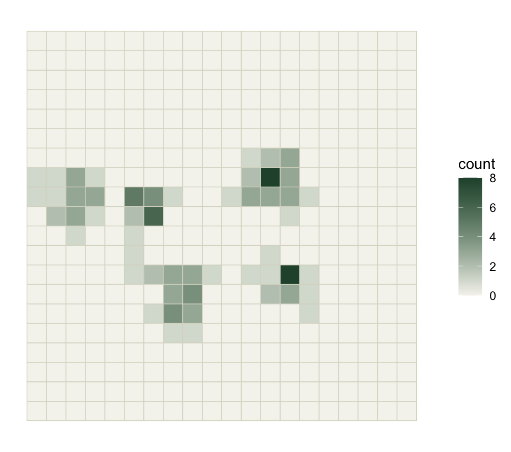
The frame is a grid of 400 quadrats. The species sits in a few tight clusters on an otherwise empty background: 87% of the quadrats are empty, and the occupancy (the fraction with at least one individual) is only 13.0%. The true quadrat mean is 0.295 individuals and the true total is 118. On a real survey you would not know these; here they are the yardstick.

Figure 1: The synthetic population. Counts are concentrated in a few clusters on an empty background, the situation adaptive cluster sampling is built for.

Under simple random sampling you would draw a fixed number of quadrats and stop. With 13% occupancy most of them are zeros, so the estimate of the mean is dominated by whether you happen to land on a cluster. Adaptive cluster sampling changes the second step: it keeps sampling around any quadrat where the species turns up.

The design: condition, neighbourhood, networks

Three ingredients define the design.

The condition decides when to expand. Here a quadrat “satisfies the condition” if its count is at least one, that is, the species is present. The neighbourhood decides where to expand: we use the four rook neighbours (up, down, left, right). The rule is then recursive. Draw an initial simple random sample; whenever a selected quadrat satisfies the condition, add its neighbours; whenever a newly added quadrat also satisfies the condition, add its neighbours too; stop when no new occupied quadrats appear.

The units partition into networks. Connected runs of occupied quadrats form one network each: selecting any one of them pulls in all of them. Every quadrat that does not satisfy the condition is a network on its own. The quadrats that sit on the boundary of a network, its non-satisfying neighbours, are the edge units: they get observed because they are adjacent to a network, but they do not trigger further expansion. build_networks() above labels the networks themselves, by a depth-first search over the occupied cells; the edge units come in later, when a draw expands around a network.

On this population there are 4 occupied networks, with sizes 19, 12, 12, 9 quadrats. Everything else is a singleton.

## one adaptive draw from an initial sample of n1 = 30 quadrats
set.seed(7)
n1 <- 30L
d1 <- acs_draw(pop, nets, ubn, n1)
c(initial = n1, distinct_networks_hit = length(d1$hit),
  final_sample = d1$n_final, naive_mean = round(d1$naive, 3))

              initial distinct_networks_hit          final_sample 
               30.000                28.000                86.000 
           naive_mean 
                0.767 

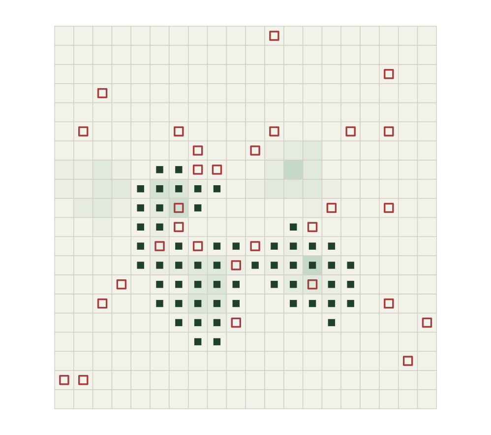
Thirty initial quadrats gave 86 observed quadrats: whenever an initial unit lands on a cluster, the whole cluster (plus its edge) comes into the sample. The plain average of everything observed in that draw was 0.767, against a truth of 0.295: the plain average of an adaptive sample is not an unbiased estimate of the population mean, because which quadrats end up observed depends on the counts themselves.

Figure 2: One adaptive draw. Open squares are the initial simple random sample; filled squares are quadrats added by expansion. Where an initial unit lands on a cluster, the whole network and its edge come in.

Why the naive mean is biased

The bias is not a fluke of one draw. Average the naive mean over many initial samples and it stays high, because expansion is triggered by high values: you always add neighbours around counts, never around empties, so the observed set is enriched for occupied quadrats relative to the frame. Formally the naive mean is not the mean of a probability sample of the frame at all, and it has no reason to be unbiased.

mc <- function(pop, nets, ubn, n1, B, seed) {
  set.seed(seed); naive <- hh <- nfin <- numeric(B); cov_hh <- logical(B)
  mu <- mean(pop$y)
  for (b in 1:B) {
    d <- acs_draw(pop, nets, ubn, n1)
    naive[b] <- d$naive; hh[b] <- d$hh; nfin[b] <- d$n_final
    se <- sqrt(max(hh_var(pop, nets, d$init, n1), 0))
    cov_hh[b] <- abs(d$hh - mu) <= 1.96 * se
  }
  list(naive = naive, hh = hh, nfin = nfin, cov_hh = cov_hh)
}
M <- mc(pop, nets, ubn, n1 = 30L, B = 20000L, seed = 202L)
c(true_mu = round(mu, 4), E_naive = round(mean(M$naive), 4),
  bias = round(mean(M$naive) - mu, 4))

true_mu E_naive    bias 
 0.2950  0.7769  0.4819 

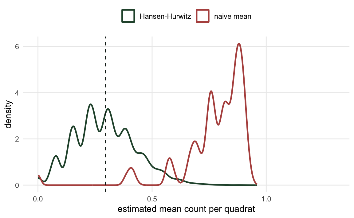
Averaged over 20,000 initial samples the naive mean is 0.7769, a bias of +0.4819, or +163%. That is not a rounding error you can ignore: the naive estimate more than doubles the truth.

The Hansen-Hurwitz estimator

The fix comes from an old idea (Hansen and Hurwitz 1943): weight each observation by how it entered the sample. In adaptive cluster sampling the clean version works through the initial units. A network is included whenever any of its units is drawn initially, and each initial draw points at exactly one network. So assign to each initial unit the mean of its network, and average those network means over the initial sample. Occupied networks contribute their cluster average; empty and edge quadrats contribute their own value (a network of one).

## Hansen-Hurwitz: mean over the initial units of their network mean
hansen_hurwitz <- function(nets, init) mean(nets$net_mean_of_unit[init])
hansen_hurwitz(nets, d1$init)          # the same draw as before

[1] 0.317739

That single draw gives 0.318, close to the truth where the naive mean gave 0.767. The estimator is design-unbiased: because the network means are defined for every unit in the frame and the initial sample is a simple random sample of those units, the Hansen-Hurwitz estimate is just the sample mean of a fixed list of 400 numbers, which is unbiased by construction.

Figure 3: Sampling distributions over 20,000 initial samples. The naive mean sits well to the right of the truth; the Hansen-Hurwitz estimator is centred on it.

Over the 20,000 samples the Hansen-Hurwitz mean is 0.2947, a bias of -0.00035: unbiased to the precision of the simulation. Its standard deviation is 0.135, against 0.146 for the naive mean, so it is both centred and tighter.

An honest limit on the interval

Unbiasedness is not the whole story. The network means are wildly skewed on a population this sparse, so the normal-based confidence interval built from the standard finite-population variance does not quite reach its nominal cover.

mean(M$cov_hh)     # cover of the nominal 95% Hansen-Hurwitz interval

[1] 0.91005

The interval covers about 91.0% of the time rather than 95%. That is the price of a rare, clumped population: the estimator is honest about the mean but the interval is optimistic, and on a real survey you would lean on a bootstrap or a design with a larger initial sample.

A second limit sits outside the interval, in the frame. The grid here misses nothing: every point of the block belongs to some quadrat. A list frame, a register of known colonies or ponds, is not like that, and the tempting conclusion is that a unit which never made the list can never be sampled. Kish’s half-open interval rule says otherwise: link each unlisted unit to the listed unit whose interval contains it, and it enters the sample whenever its linking unit does, with that unit’s known, non-zero inclusion probability. What the rule costs is area rather than visits. In the plane the interval becomes the ground a listed unit owns, which on a frame like this one is its own quadrat, and honouring the link means sweeping that ground instead of checking the listed unit sitting in it. On a frame that tiles the block, as this one does, the two jobs coincide: no unit is unlisted, so the rule asks for nothing beyond the ground the design already owes, and the two figures that follow price the adaptive expansion itself rather than the linking. Adaptive expansion then enlarges the bill, because a network mean depends on every unit of the network and its edge, so the sweep has to cover the whole final sample: 24.2% of the block on this design, against 7.5% if the initial draw were all you had to sweep. An unlisted unit is not out of reach, then, but reaching it is priced in ground covered, and the price rises with the same expansion that makes the design efficient.

The next post keeps the same design but swaps the estimator for the Horvitz-Thompson version, which uses the network inclusion probabilities directly and buys back some of that precision.

References

Hansen MH, Hurwitz WN 1943 Ann Math Stat 14(4):333-362 (10.1214/aoms/1177731356)

Thompson SK 1990 J Am Stat Assoc 85(412):1050-1059 (10.1080/01621459.1990.10474975)

Smith DR, Conroy MJ, Brakhage DH 1995 Biometrics 51(2):777-788 (10.2307/2532964)

Thompson SK, Seber GAF 1996 Adaptive Sampling. Wiley (ISBN 978-0-471-55871-2)

Related tutorials

• Horvitz-Thompson for adaptive samples
• When does adaptive sampling pay?
• Checking an adaptive sampling design
• Stratified random sampling in ecology