---
title: "Stratified random sampling in ecology"
description: "Stratified random sampling in R from first principles: the weighted estimator, its design variance, and why splitting a landscape into strata sharpens a mean."
date: "2026-06-26 13:00"
categories: [R, survey design, sampling, ecology tutorial]
image: thumbnail.png
image-alt: "Sampling distributions of a simple random sample mean and a stratified mean, the stratified one much narrower"
date-modified: "2026-10-14"
---
*Corrected 14 October 2026: the post stated its rule, that stratification removes the between-stratum variance and nothing else, and its verdict that strata which do not separate the response are decoration, as if they held for any split of the effort; both hold under proportional allocation, the post now says so, and it adds that strata whose spreads differ can still gain through the allocation.*
*Corrected 7 October 2026: the section on the honest limit called stratification optimal for the variable stratified on, which nothing in the post shows; it now says that stratification sharpens the estimate of a variable whose means differ between the strata.*
*Corrected 27 September 2026: the number of random plots needed to match the stratified design was given as 371, which ignored the finite population correction; with it included the figure is 307.*
Walk any real landscape and the variation is not spread evenly. A wet hollow carries several times the biomass of the dry woodland floor next to it, and the two barely overlap. If you scatter plots at random over the whole area, most of the spread in your data comes from the fact that some plots landed in one habitat and some in the other. That spread is not news. You knew where the habitats were before you started.
Stratified sampling turns that prior knowledge into precision. You split the frame into strata, sample inside each one separately, and put the pieces back together with weights you already know. The estimator stays design based: no model, no assumption about the shape of anything, just the sampling plan you followed.
This post builds the estimator and its variance by hand, checks both against a simulation, and then shows the case where stratification with proportional allocation buys nothing at all.
## A frame you can count
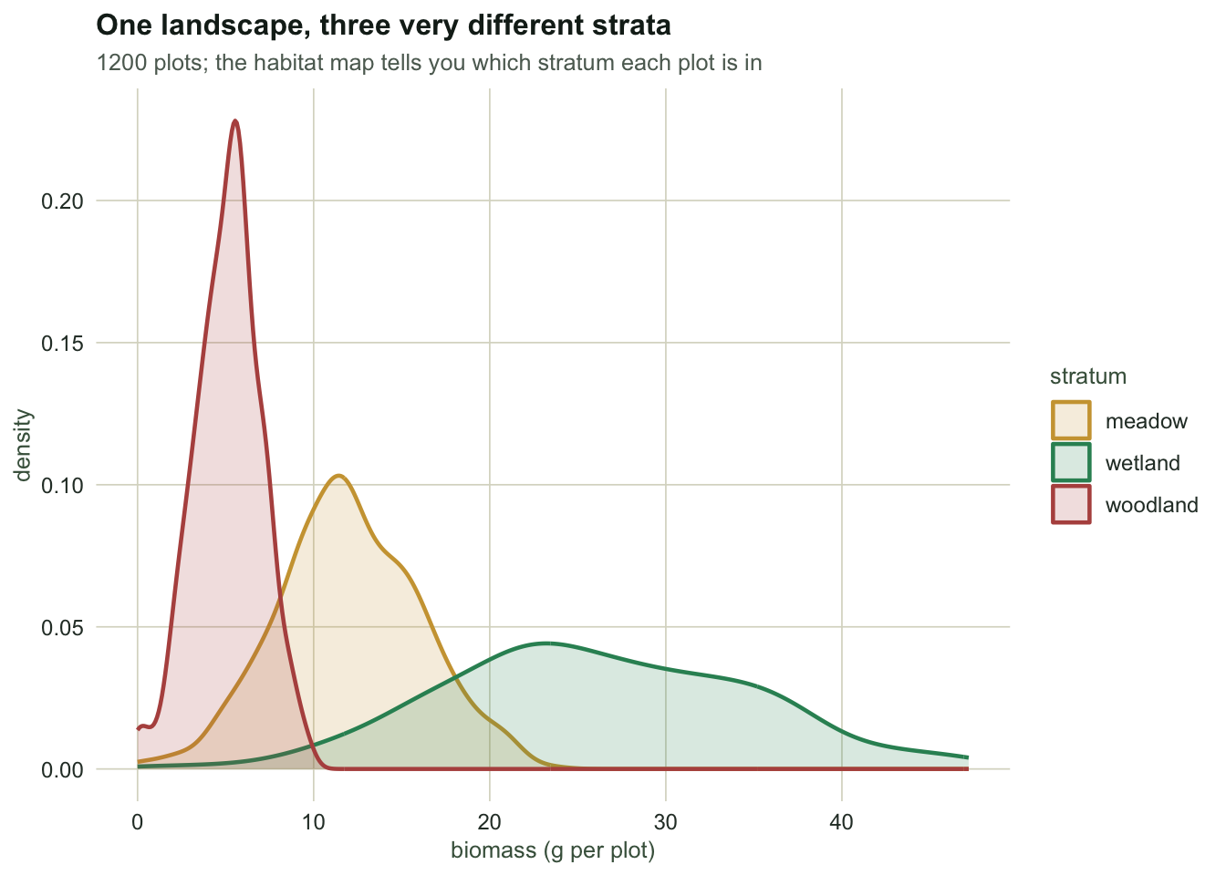
The landscape is 1200 plots in three habitat strata. Their sizes are known from a habitat map, which is the whole point: the weights come from the frame, not from the sample.
```{r frame}
set.seed(371)

Nh   <- c(meadow = 600, wetland = 300, woodland = 300)
mu_h <- c(meadow = 12,  wetland = 26,  woodland = 5)
sd_h <- c(meadow = 4,   wetland = 9,   woodland = 2)

N       <- sum(Nh)
H       <- length(Nh)
stratum <- rep(names(Nh), Nh)
y       <- round(pmax(0, rnorm(N, rep(mu_h, Nh), rep(sd_h, Nh))), 2)

W   <- Nh / N                                    # stratum weights, known
mu  <- mean(y)                                   # population mean (we get to peek)
S2  <- var(y)                                    # population variance, divisor N - 1
S2h <- tapply(y, stratum, var)[names(Nh)]        # within-stratum variances
muh <- tapply(y, stratum, mean)[names(Nh)]
round(rbind(W = W, mean = muh, sd = sqrt(S2h)), 3)
```
```{r fig-frame}
#| echo: false
#| fig-cap: "Plot-level biomass in the three strata. The wetland sits well above the meadow, the woodland well below, and the wetland is also the most variable stratum."
#| fig-alt: "Three overlaid density curves for meadow, wetland and woodland biomass. Woodland is a narrow peak near five, meadow a moderate peak near twelve, wetland a broad curve near twenty six."
library(ggplot2)
theme_te <- function() {
theme_minimal(base_size = 11) +
theme(
plot.background = element_rect(fill = "#f5f4ee", colour = NA),
panel.background = element_rect(fill = "#f5f4ee", colour = NA),
panel.grid.minor = element_blank(),
panel.grid.major = element_line(colour = "#dad9ca", linewidth = 0.3),
plot.title = element_text(colour = "#16241d", face = "bold", size = 12),
plot.subtitle = element_text(colour = "#5d6b61", size = 9.5),
axis.title = element_text(colour = "#46604a", size = 9.5),
axis.text = element_text(colour = "#2c3a31", size = 9),
legend.title = element_text(colour = "#46604a", size = 9.5),
legend.text = element_text(colour = "#2c3a31", size = 9),
strip.text = element_text(colour = "#16241d", face = "bold", size = 10)
)
}
pal_h <- c(meadow = "#cda23f", wetland = "#2f8f63", woodland = "#b5534e")
ggplot(data.frame(y = y, stratum = factor(stratum, levels = names(Nh))),
aes(y, colour = stratum, fill = stratum)) +
geom_density(alpha = 0.18, linewidth = 0.8) +
scale_colour_manual(values = pal_h) +
scale_fill_manual(values = pal_h) +
labs(title = "One landscape, three very different strata",
subtitle = "1200 plots; the habitat map tells you which stratum each plot is in",
x = "biomass (g per plot)", y = "density",
colour = "stratum", fill = "stratum") +
theme_te()
```
## Two estimators for the same mean
A simple random sample of `n` plots estimates the mean with the plain sample mean. Its design variance is the textbook one, finite population correction included:
$$V_{\text{srs}}(\bar y) = \left(1 - \tfrac{n}{N}\right)\frac{S^2}{n}.$$
A stratified sample takes $n_h$ plots inside stratum $h$ and combines the stratum means with the known weights, $\bar y_{\text{st}} = \sum_h W_h \bar y_h$. Because the strata are sampled independently, the variances simply add:
$$V_{\text{st}}(\bar y_{\text{st}}) = \sum_h W_h^2 \left(1 - \tfrac{n_h}{N_h}\right)\frac{S_h^2}{n_h}.$$
With a budget of 120 plots and effort split in proportion to stratum size:
```{r estimators}
n  <- 120
f  <- n / N
nh <- round(n * W)                                # proportional allocation
nh
V_srs  <- (1 - f) * S2 / n
V_prop <- sum(W^2 * (1 - nh / Nh) * S2h / nh)
c(SE_srs = sqrt(V_srs), SE_stratified = sqrt(V_prop), ratio = V_srs / V_prop)
```
```{r scalars-1}
#| echo: false
se_srs <- sqrt(V_srs)
se_str <- sqrt(V_prop)
deff <- V_srs / V_prop
n_equiv <- ceiling(1 / (V_prop / S2 + 1 / N)) # SRS size with the same variance, FPC included
```
The stratified standard error is `r sprintf("%.3f", se_str)` against `r sprintf("%.3f", se_srs)` for the simple random sample, a variance ratio of `r sprintf("%.2f", deff)`. To match the stratified design with random plots you would need about `r n_equiv` plots instead of `r n` (fewer than the variance ratio times `r n`, because the finite population correction also tightens as the random sample grows), for the same field season, on the same landscape, measuring the same thing. The only extra input was the habitat map.
## Where the gain comes from
Split the population variance into a within part and a between part. The identity is exact for a finite population:
$$(N-1)S^2 = \sum_h (N_h - 1) S_h^2 + \sum_h N_h (\mu_h - \mu)^2.$$
```{r decomposition}
within  <- sum((Nh - 1) * S2h) / (N - 1)
between <- sum(Nh * (muh - mu)^2) / (N - 1)
c(S2 = S2, within = within, between = between,
  check = within + between - S2, between_share = between / S2)
```
```{r scalars-2}
#| echo: false
share_between <- between / S2
gap_within <- within - sum(W * S2h)
```
`r sprintf("%.1f", 100 * share_between)` per cent of the total variance lives between the strata. Now compare the two design variances under proportional allocation, where $n_h/N_h$ equals $n/N$ in every stratum:
$$V_{\text{srs}} - V_{\text{st}} = \frac{1-f}{n}\left(S^2 - \sum_h W_h S_h^2\right).$$
The bracket is the between-stratum component, up to a finite population bookkeeping term of order $1/N$ (here the two versions differ by `r sprintf("%.3f", abs(gap_within))`, against a total variance of `r sprintf("%.1f", S2)`). So the rule for proportional allocation is short: **stratification removes the between-stratum variance from your error, and nothing else.** What it leaves out is how the effort is split between the strata, which the last section comes back to.
## Does the arithmetic survive a simulation?
Formulas for design variance are easy to write and easy to get wrong. Draw the samples and look.
```{r monte-carlo}
idx_h <- split(seq_len(N), stratum)[names(Nh)]
B     <- 4000

draw_srs <- function() mean(y[sample.int(N, n)])
draw_str <- function() sum(W * vapply(seq_len(H), function(h)
                        mean(y[sample(idx_h[[h]], nh[h])]), 0))

set.seed(3711); mc_srs <- replicate(B, draw_srs())
set.seed(3712); mc_str <- replicate(B, draw_str())

rbind(simple     = c(mean = mean(mc_srs), variance = var(mc_srs), analytic = V_srs),
      stratified = c(mean = mean(mc_str), variance = var(mc_str), analytic = V_prop))
```
```{r scalars-3}
#| echo: false
mc_v_srs <- var(mc_srs); mc_v_str <- var(mc_str)
```
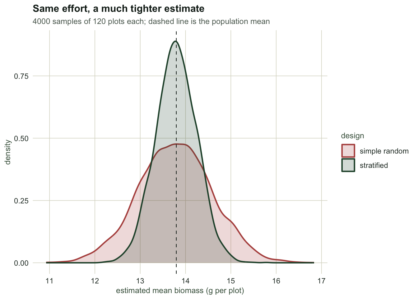
Both estimators centre on the true mean of `r sprintf("%.2f", mu)`, and both simulated variances land on their formulas: `r sprintf("%.3f", mc_v_srs)` against `r sprintf("%.3f", V_srs)`, and `r sprintf("%.3f", mc_v_str)` against `r sprintf("%.3f", V_prop)`.
```{r fig-sampling}
#| echo: false
#| fig-cap: "Sampling distributions of the two estimators over 4000 draws, same 120 plots of effort. Both are centred on the population mean; the stratified one is far narrower."
#| fig-alt: "Two overlaid density curves of estimated means. The simple random sample curve is wide, the stratified curve is roughly half as wide, both centred on the same value."
dd <- rbind(data.frame(est = mc_srs, design = "simple random"),
data.frame(est = mc_str, design = "stratified"))
ggplot(dd, aes(est, colour = design, fill = design)) +
geom_density(alpha = 0.2, linewidth = 0.8) +
geom_vline(xintercept = mu, colour = "#16241d", linetype = "dashed", linewidth = 0.4) +
scale_colour_manual(values = c("simple random" = "#b5534e", "stratified" = "#275139")) +
scale_fill_manual(values = c("simple random" = "#b5534e", "stratified" = "#275139")) +
labs(title = "Same effort, a much tighter estimate",
subtitle = "4000 samples of 120 plots each; dashed line is the population mean",
x = "estimated mean biomass (g per plot)", y = "density",
colour = "design", fill = "design") +
theme_te()
```
## The variance estimator you actually report
In the field you do not know $S_h^2$. You estimate it from the sample, stratum by stratum, and plug it in. That estimator is unbiased, and the interval it produces covers at the nominal rate:
```{r variance-estimator}
one_survey <- function() {
  s   <- lapply(seq_len(H), function(h) y[sample(idx_h[[h]], nh[h])])
  est <- sum(W * vapply(s, mean, 0))
  v   <- sum(W^2 * (1 - nh / Nh) * vapply(s, var, 0) / nh)
  c(estimate = est, variance = v)
}

set.seed(3713)
surveys  <- t(replicate(B, one_survey()))
coverage <- mean(abs(surveys[, "estimate"] - mu) <= 1.96 * sqrt(surveys[, "variance"]))
c(mean_v_hat = mean(surveys[, "variance"]), true_V = V_prop, coverage = coverage)
```
```{r scalars-4}
#| echo: false
v_hat_mean <- mean(surveys[, "variance"]); cov_str <- coverage
```
The average estimated variance is `r sprintf("%.4f", v_hat_mean)` against a true `r sprintf("%.4f", V_prop)`, and `r sprintf("%.1f", 100 * cov_str)` per cent of the intervals caught the mean. Nothing here leans on normality of the plot values; it leans on the central limit theorem applied inside each stratum, which is why very small $n_h$ is a problem worth a post of its own.
## When stratification buys nothing
Under proportional allocation the gain is the between-stratum variance. Take that away and the gain goes with it. Shift each stratum onto the common mean, leaving the within-stratum spread untouched, and re-run the same arithmetic:
```{r flat-frame}
y_flat <- y
for (h in names(Nh)) y_flat[stratum == h] <- y[stratum == h] - muh[h] + mu

S2_flat  <- var(y_flat)
S2h_flat <- tapply(y_flat, stratum, var)[names(Nh)]
c(V_srs = (1 - f) * S2_flat / n,
  V_str = sum(W^2 * (1 - nh / Nh) * S2h_flat / nh),
  ratio = ((1 - f) * S2_flat / n) / sum(W^2 * (1 - nh / Nh) * S2h_flat / nh))
```
```{r scalars-5}
#| echo: false
ratio_flat <- ((1 - f) * S2_flat / n) / sum(W^2 * (1 - nh / Nh) * S2h_flat / nh)
```
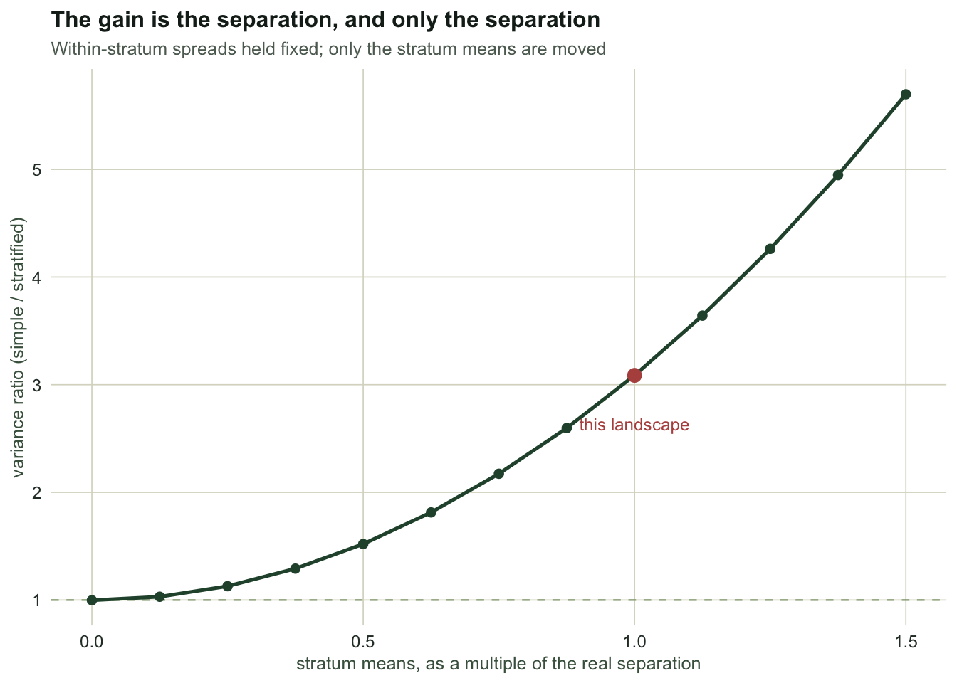
The ratio is `r sprintf("%.3f", ratio_flat)`. The wetland is still `r sprintf("%.1f", sqrt(S2h[["wetland"]] / S2h[["woodland"]]))` times as variable as the woodland, the map is still correct, the allocation is still proportional, and the design has gained nothing measurable. Under proportional allocation, strata that do not separate the response are decoration; when their spreads differ this much, an allocation that follows the spreads can still gain, as the last section suggests.
Sweeping the separation from zero up to one and a half times the real gaps shows the whole curve:
```{r sweep}
k_grid <- seq(0, 1.5, by = 0.125)
ratio_k <- vapply(k_grid, function(k) {
  yk <- y
  for (h in names(Nh))
    yk[stratum == h] <- y[stratum == h] - muh[h] + mu + k * (muh[h] - mu)
  S2k  <- var(yk)
  S2hk <- tapply(yk, stratum, var)[names(Nh)]
  ((1 - f) * S2k / n) / sum(W^2 * (1 - nh / Nh) * S2hk / nh)
}, 0)
setNames(round(ratio_k, 2), k_grid)
```
```{r fig-sweep}
#| echo: false
#| fig-cap: "Variance ratio against how far apart the stratum means are, as a multiple of the real separation. At zero separation the ratio is one: identical within-stratum spreads, identical precision."
#| fig-alt: "Rising curve of variance ratio against stratum mean separation. It starts at one when the means coincide and climbs past five at one and a half times the real separation."
ggplot(data.frame(k = k_grid, ratio = ratio_k), aes(k, ratio)) +
geom_hline(yintercept = 1, colour = "#93a87f", linetype = "dashed", linewidth = 0.4) +
geom_line(colour = "#275139", linewidth = 0.9) +
geom_point(colour = "#275139", size = 1.9) +
annotate("point", x = 1, y = ratio_k[k_grid == 1], colour = "#b5534e", size = 3) +
annotate("text", x = 1, y = ratio_k[k_grid == 1] - 0.45, label = "this landscape",
colour = "#b5534e", size = 3.2) +
labs(title = "Under proportional allocation, the gain is the separation",
subtitle = "Within-stratum spreads held fixed; only the stratum means are moved",
x = "stratum means, as a multiple of the real separation",
y = "variance ratio (simple / stratified)") +
theme_te()
```
## The honest limit
Stratification sharpens the estimate of a variable whose means differ between the strata, and of no other variable automatically. A partition that separates biomass may cut straight across the gradient that drives species richness, in which case the richness estimate gains nothing while the biomass estimate gains a factor of `r sprintf("%.1f", deff)`. Surveys usually carry more than one response, and the strata are one decision serving all of them.
Two further conditions do real work and both are about the frame rather than the statistics. The stratum sizes $N_h$ have to be the true sizes of the sets you sampled from, because they enter the estimator directly. And every plot has to belong to exactly one stratum with a known, non-zero chance of selection. Get either wrong and the estimator stops being unbiased, which is a different kind of problem from being imprecise.
## Where to go next
Proportional allocation is the safe default, not the best one. The wetland here is `r sprintf("%.1f", sqrt(S2h[["wetland"]] / S2h[["woodland"]]))` times as variable as the woodland, and sending equal fractions of effort to both is leaving precision on the table. The next post works out the allocation that minimises the variance, what it costs when a stratum is expensive to reach, and how much of the promised gain survives being planned from a small pilot.
## References
Neyman 1934 J R Stat Soc 97(4):558-625 (10.2307/2342192)
Cochran 1977 Sampling Techniques, 3rd edn, Wiley; ISBN 978-0-471-16240-7
Sarndal, Swensson and Wretman 1992 Model Assisted Survey Sampling, Springer; ISBN 978-0-387-40620-6
Thompson 2012 Sampling, 3rd edn, Wiley; ISBN 978-0-470-40231-3
Gregoire and Valentine 2008 Sampling Strategies for Natural Resources and the Environment, Chapman and Hall; ISBN 978-1-58488-370-8
## Related tutorials
- [Allocating survey effort across strata](../allocating-effort-across-strata/)
- [Two-phase sampling when strata are unknown](../two-phase-sampling-for-stratification/)
- [Checking a stratified design](../checking-a-stratified-design/)
- [Spatially balanced sampling with GRTS](../spatially-balanced-sampling-and-grts/)