---
title: "Two-phase sampling when strata are unknown"
description: "Double sampling in R: a large cheap first phase builds the strata, a small expensive second phase measures the response, and the budget split follows a formula."
date: "2026-06-27 09:00"
date-modified: "2026-10-15"
categories: [R, survey design, sampling, ecology tutorial]
image: thumbnail.png
image-alt: "U-shaped curve of design variance against the share of budget spent on the cheap first phase, with the optimum marked"
---
*Corrected 15 October 2026: the closing section still called the variance formula an approximation for large phase-one stratum counts; it now says the formula is exact apart from rounding the subsample sizes. The budget rule now speaks of units rather than spending, because raising a phase's unit cost lowers its number of units but raises its share of the budget, and the subtitle of the design comparison no longer suggests that a simple random sample needs a map.*
*Corrected 7 October 2026: the post said that subsampling in proportion to the stratum standard deviations is free, using information the first phase has already collected; it now says the gain assumes the true standard deviations of the response, which the cheap first phase does not record. It also called the variance formula a large-sample approximation, where with a common subsampling fraction it is exact apart from rounding the subsample sizes, and the budget and cost curves no longer include designs that cannot be run.*
Stratified sampling assumes a map. You need to know which stratum every plot belongs to and how large each stratum is, before a single measurement is taken. Plenty of surveys have no such map: the habitat classification is exactly what you would have to go out and produce, and by then you have spent the season.
Two-phase sampling, also called double sampling, buys the map with part of the budget. Phase one visits a large sample and records something cheap: a habitat call from the track, a canopy class, a rapid cover estimate. Phase two returns to a subsample of those units and does the expensive thing: harvesting, weighing, sorting, sequencing. The cheap phase supplies the stratum weights, the expensive phase supplies the stratum means, and the two are combined into one estimate.
The interesting part is that the variance splits neatly along the same seam, which turns the budget split into arithmetic instead of a hunch.
## The setup
Same landscape, but now nobody has the habitat map:
```{r frame}
set.seed(371)

Nh   <- c(meadow = 600, wetland = 300, woodland = 300)
mu_h <- c(meadow = 12,  wetland = 26,  woodland = 5)
sd_h <- c(meadow = 4,   wetland = 9,   woodland = 2)

N       <- sum(Nh)
stratum <- rep(names(Nh), Nh)
y       <- round(pmax(0, rnorm(N, rep(mu_h, Nh), rep(sd_h, Nh))), 2)

W   <- Nh / N
mu  <- mean(y)
S2  <- var(y)
S2h <- tapply(y, stratum, var)[names(Nh)]

within  <- sum(W * S2h)          # what stays inside the strata
between <- S2 - within           # what the strata remove
c(total = S2, between = between, within = within)
```
```{r scalars-0}
#| echo: false
share_between <- between / S2
```
`r sprintf("%.0f", 100 * share_between)` per cent of the variance sits between the strata and the rest sits inside them. Hold on to those two numbers, because they turn out to be the price tags of the two phases.
## The estimator
Draw a simple random sample of `n1` units and record the cheap classification. That gives estimated weights $w_h = n_{1h}/n_1$. Then subsample each phase-one stratum and measure the response, giving $\bar y_h$. The estimator is the same weighted sum as before, with estimated weights in place of known ones:
$$\bar y_{\text{2ph}} = \sum_h w_h \bar y_h .$$
It is unbiased. Conditional on the phase-one sample, the expectation is the phase-one sample mean of the response, and the phase-one sample mean is unbiased for the population mean, so the two steps compose.
## The variance splits along the phases
Condition on phase one and add the two pieces. The variation of the phase-one mean contributes $(1 - n_1/N)S^2/n_1$; the subsampling contributes the usual within-stratum term, evaluated at the phase-two sizes. Written with a common subsampling fraction it collapses to
$$V(\bar y_{\text{2ph}}) \;\approx\; \Big(1 - \tfrac{n_1}{N}\Big)\frac{S^2}{n_1} \;+\; \Big(\sum_h W_h S_h^2\Big)\left(\frac{1}{n_2} - \frac{1}{n_1}\right),$$
and, ignoring the finite population correction, into something worth putting on a wall:
$$V \;\approx\; \frac{\text{between}}{n_1} \;+\; \frac{\text{within}}{n_2}.$$
**The cheap phase pays for the between-stratum variance and the expensive phase pays for the within-stratum variance.** That is the whole design in one line.
```{r variance-fn}
V_2ph <- function(n1, n2) (1 - n1 / N) * S2 / n1 + within * (1 / n2 - 1 / n1)
c(`n1=400, n2=100` = V_2ph(400, 100), `n1=300, n2=60` = V_2ph(300, 60))
```
## Does the formula hold?
Simulate the whole two-phase procedure, weights and all, and compare.
```{r monte-carlo}
one_survey <- function(n1, n2) {
  s1 <- sample.int(N, n1)
  st <- stratum[s1]
  w  <- table(factor(st, levels = names(Nh))) / n1
  nu <- n2 / n1
  est <- 0
  for (h in names(Nh)) {
    ix <- s1[st == h]
    est <- est + w[[h]] * mean(y[sample(ix, max(1, round(nu * length(ix))))])
  }
  est
}

B <- 3000
res <- t(sapply(list(c(400, 100), c(300, 60)), function(p) {
  set.seed(3731)
  mc <- replicate(B, one_survey(p[1], p[2]))
  c(n1 = p[1], n2 = p[2], mc_mean = mean(mc), truth = mu,
    mc_variance = var(mc), formula = V_2ph(p[1], p[2]))
}))
round(res, 4)
```
```{r scalars-1}
#| echo: false
mc_v1 <- res[1, "mc_variance"]; fo_v1 <- res[1, "formula"]
mc_b1 <- res[1, "mc_mean"] - mu
rel1 <- 100 * (fo_v1 / mc_v1 - 1)
```
The simulated variance is `r sprintf("%.3f", mc_v1)` against a predicted `r sprintf("%.3f", fo_v1)`. With a common subsampling fraction the formula is exact apart from rounding the subsample sizes to whole units, so the gap between the two is simulation noise: what to check is whether they sit close, not which way the difference falls. The estimator itself is centred, with a simulated bias of `r sprintf("%.3f", mc_b1)` on a mean of `r sprintf("%.2f", mu)`.
## Splitting a budget
Let phase one cost $c_1$ per unit and phase two cost $c_2$, and fix the total. Minimising $A/n_1 + B/n_2$ under $c_1 n_1 + c_2 n_2 = C$ is a one-line Lagrange problem with a memorable answer,
$$\frac{n_1}{n_2} = \sqrt{\frac{A\,c_2}{B\,c_1}},$$
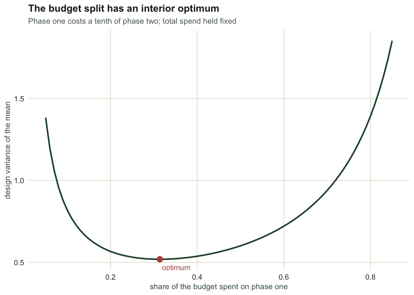
where $A$ is the between-stratum component and $B$ the within-stratum one. Put more units into the phase that is buying the larger piece of variance, and fewer into the phase whose units cost more.
```{r budget-split}
c1 <- 1; c2 <- 10; budget <- 1000

ratio <- sqrt(between * c2 / (within * c1))
n2_opt <- budget / (ratio * c1 + c2)
n1_opt <- ratio * n2_opt
c(n1 = n1_opt, n2 = n2_opt, V = V_2ph(n1_opt, n2_opt), SE = sqrt(V_2ph(n1_opt, n2_opt)))
```
```{r fig-split}
#| echo: false
#| fig-cap: "Design variance against how the budget is divided, holding total spend fixed. Too little phase one and the weights are noisy; too much and there is nothing left to measure the response with."
#| fig-alt: "U-shaped curve of design variance against the share of budget spent on phase one, with a minimum around one third and a marked optimum point."
library(ggplot2)
theme_te <- function() {
theme_minimal(base_size = 11) +
theme(
plot.background = element_rect(fill = "#f5f4ee", colour = NA),
panel.background = element_rect(fill = "#f5f4ee", colour = NA),
panel.grid.minor = element_blank(),
panel.grid.major = element_line(colour = "#dad9ca", linewidth = 0.3),
plot.title = element_text(colour = "#16241d", face = "bold", size = 12),
plot.subtitle = element_text(colour = "#5d6b61", size = 9.5),
axis.title = element_text(colour = "#46604a", size = 9.5),
axis.text = element_text(colour = "#2c3a31", size = 9),
legend.title = element_text(colour = "#46604a", size = 9.5),
legend.text = element_text(colour = "#2c3a31", size = 9),
strip.text = element_text(colour = "#16241d", face = "bold", size = 10)
)
}
sh <- seq(0.1, 0.85, by = 0.01)
cv <- data.frame(share = sh,
V = vapply(sh, function(s) V_2ph(budget * s / c1, budget * (1 - s) / c2), 0))
ggplot(cv, aes(share, V)) +
geom_line(colour = "#275139", linewidth = 0.9) +
annotate("point", x = n1_opt * c1 / budget, y = V_2ph(n1_opt, n2_opt),
colour = "#b5534e", size = 3) +
annotate("text", x = n1_opt * c1 / budget, y = V_2ph(n1_opt, n2_opt),
label = " optimum", hjust = 0, vjust = -1, colour = "#b5534e", size = 3.2) +
labs(title = "The budget split has an interior optimum",
subtitle = "Phase one costs a tenth of phase two; total spend held fixed",
x = "share of the budget spent on phase one",
y = "design variance of the mean") +
theme_te()
```
## What the design is worth
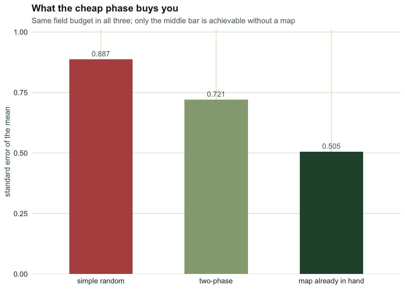
Three ways to spend the same money. Spend it all on the expensive measurement and take a simple random sample. Split it between the phases. Or, the unattainable benchmark, have the map already and run a proper stratified survey.
```{r three-way}
n_srs <- budget / c2
V_srs <- (1 - n_srs / N) * S2 / n_srs
V_map <- (1 - n_srs / N) / n_srs * within        # stratified, weights known in advance

comparison <- rbind(
  `simple random`  = c(expensive_units = n_srs, V = V_srs,                SE = sqrt(V_srs)),
  `two-phase`      = c(expensive_units = n2_opt, V = V_2ph(n1_opt, n2_opt),
                       SE = sqrt(V_2ph(n1_opt, n2_opt))),
  `map already in hand` = c(expensive_units = n_srs, V = V_map,           SE = sqrt(V_map)))
round(comparison, 4)
```
```{r scalars-2}
#| echo: false
gap_closed <- (V_srs - V_2ph(n1_opt, n2_opt)) / (V_srs - V_map)
se_srs <- sqrt(V_srs); se_2ph <- sqrt(V_2ph(n1_opt, n2_opt)); se_map <- sqrt(V_map)
```
```{r fig-three}
#| echo: false
#| fig-cap: "Standard error on an identical budget. Two-phase sampling recovers part of the distance between a simple random sample and a survey that already had the map, and it recovers it without a map."
#| fig-alt: "Three bars of standard error: simple random highest, two-phase in the middle, map-in-hand stratified lowest."
cd <- data.frame(design = factor(rownames(comparison), levels = rownames(comparison)),
SE = comparison[, "SE"])
ggplot(cd, aes(design, SE)) +
geom_col(fill = c("#b5534e", "#93a87f", "#275139"), width = 0.55) +
geom_text(aes(label = sprintf("%.3f", SE)), vjust = -0.6, colour = "#5d6b61", size = 3.2) +
scale_y_continuous(expand = expansion(mult = c(0, 0.14))) +
labs(title = "What the cheap phase buys you",
subtitle = "Same field budget in all three; only the right-hand bar needs a map in advance",
x = NULL, y = "standard error of the mean") +
theme_te()
```
Two-phase sampling closes `r sprintf("%.0f", 100 * gap_closed)` per cent of the variance gap between having no map and having one, standard error `r sprintf("%.3f", se_2ph)` against `r sprintf("%.3f", se_srs)` and `r sprintf("%.3f", se_map)`. Buying the map with survey effort is worth doing, and it is not the same as being handed one.
## When the cheap phase is not cheap enough
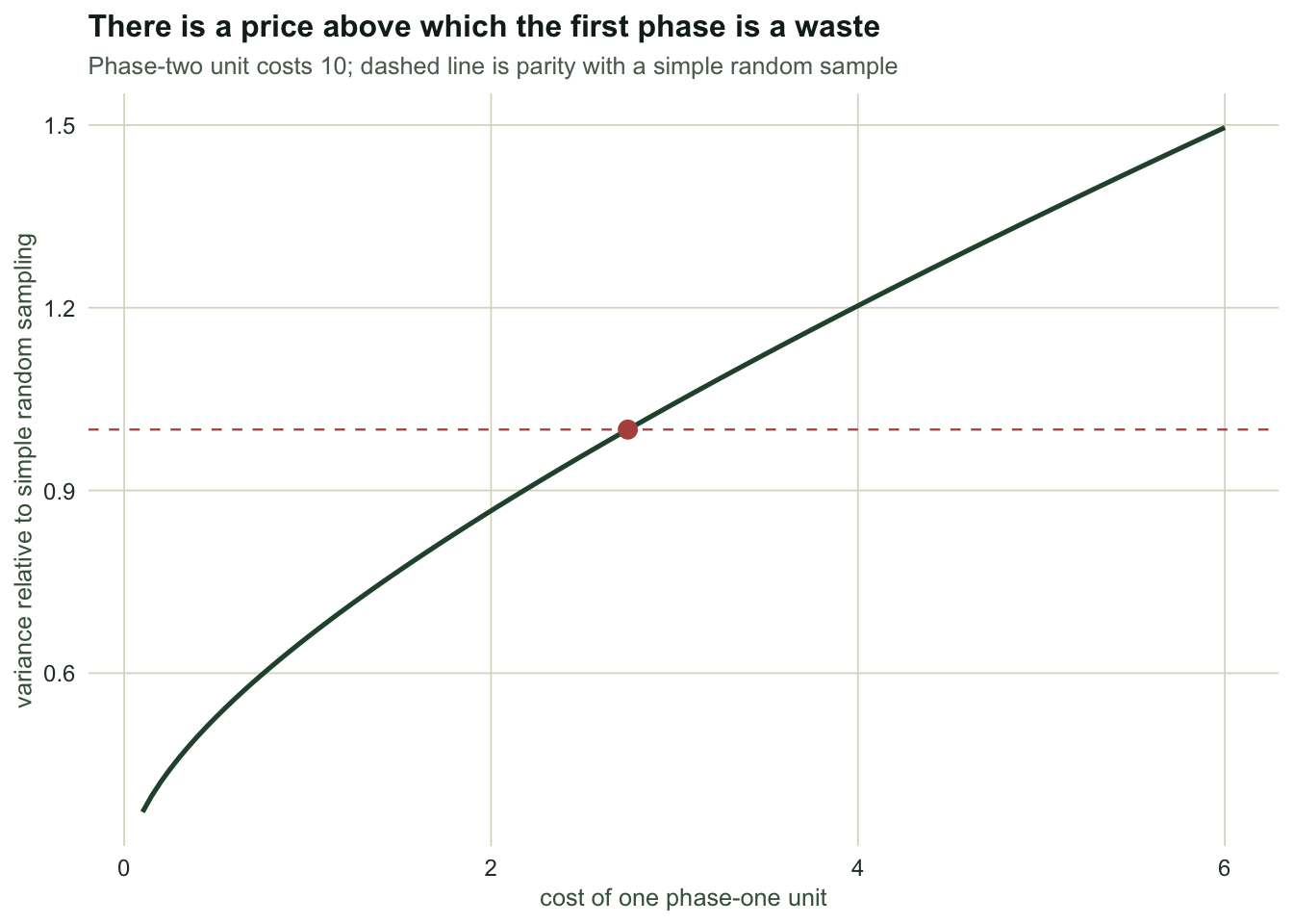
All of that depends on $c_1$. Push the first phase towards the price of the second and the design stops paying for itself, because every phase-one unit is a phase-two unit you did not buy.
```{r cost-sweep}
V_at <- function(cc) {
  r <- sqrt(between * c2 / (within * cc))
  n2 <- budget / (r * cc + c2)
  V_2ph(r * n2, n2)
}
break_even <- uniroot(function(cc) V_at(cc) - V_srs, c(0.2, 20))$root

sweep <- data.frame(c1 = c(0.2, 0.5, 1, 2, 4))
sweep$V     <- vapply(sweep$c1, V_at, 0)
sweep$ratio <- sweep$V / V_srs
round(sweep, 4)
c(break_even_c1 = break_even, as_fraction_of_c2 = break_even / c2)
```
```{r scalars-3}
#| echo: false
be_frac <- break_even / c2
```
The break-even point is a phase-one unit costing `r sprintf("%.0f", 100 * be_frac)` per cent of a phase-two unit. Below that, two phases beat one; above it, you should have spent everything on the response. In this landscape the classification would have to be genuinely quick, a call from the vehicle rather than a walked transect.
```{r fig-cost}
#| echo: false
#| fig-cap: "Two-phase variance relative to a simple random sample, as the cost of a phase-one unit rises. The design pays for itself only to the left of the crossing point."
#| fig-alt: "Rising curve of relative variance against phase-one cost, crossing the value one just before a phase-one cost of three."
cs <- seq(0.15, 6, by = 0.05)
cd2 <- data.frame(c1 = cs, ratio = vapply(cs, function(cc) V_at(cc) / V_srs, 0))
ggplot(cd2, aes(c1, ratio)) +
geom_hline(yintercept = 1, colour = "#b5534e", linetype = "dashed", linewidth = 0.4) +
geom_line(colour = "#275139", linewidth = 0.9) +
annotate("point", x = break_even, y = 1, colour = "#b5534e", size = 3) +
labs(title = "There is a price above which the first phase is a waste",
subtitle = "Phase-two unit costs 10; dashed line is parity with a simple random sample",
x = "cost of one phase-one unit", y = "variance relative to simple random sampling") +
theme_te()
```
## Two refinements worth knowing
The subsampling fraction does not have to be the same in every stratum. Minimising the same variance with $\nu_h$ free gives the Neyman analogue, $\nu_h \propto S_h$, and the within term becomes $(\sum_h W_h S_h)^2/n_2$:
```{r optimal-nu}
Sh <- sqrt(S2h)
V_2ph_opt <- function(n1, n2) (1 - n1 / N) * S2 / n1 + (sum(W * Sh))^2 / n2 - within / n1
r2  <- sqrt(between * c2 / ((sum(W * Sh))^2 * c1))
n2b <- budget / (r2 * c1 + c2); n1b <- r2 * n2b
c(n1 = n1b, n2 = n2b, V_uniform = V_2ph(n1_opt, n2_opt), V_optimal_nu = V_2ph_opt(n1b, n2b))
```
```{r scalars-4}
#| echo: false
nu_gain <- 1 - V_2ph_opt(n1b, n2b) / V_2ph(n1_opt, n2_opt)
```
Subsampling in proportion to the stratum standard deviations takes another `r sprintf("%.0f", 100 * nu_gain)` per cent off the variance on the same budget. It is the same Neyman argument one level down, and it needs the same input: that figure uses the true standard deviations of the response in each stratum, which the cheap first phase does not record, so in practice they have to come from a pilot or an earlier survey.
The second refinement is a warning. The phase-one classification is allowed to be wrong. Because the estimator weights whatever classes the field call produced, misclassification does not bias anything; it only makes the classes separate the response less well, which shows up as a smaller between component.
```{r proxy-error}
set.seed(3733)
proxy <- do.call(rbind, lapply(c(0, 0.10, 0.20, 0.35), function(e) {
  cls <- stratum
  flip <- runif(N) < e
  cls[flip] <- sample(names(Nh), sum(flip), replace = TRUE)
  Wc  <- as.numeric(table(factor(cls, levels = names(Nh)))) / N
  wi  <- sum(Wc * tapply(y, cls, var)[names(Nh)])
  r   <- sqrt((S2 - wi) * c2 / (wi * c1)); n2e <- budget / (r * c1 + c2); n1e <- r * n2e
  Ve  <- (1 - n1e / N) * S2 / n1e + wi * (1 / n2e - 1 / n1e)
  data.frame(error = e, within_share = wi / S2, V = Ve, ratio_to_srs = Ve / V_srs)
}))
round(proxy, 3)
```
```{r scalars-5}
#| echo: false
r10 <- proxy$ratio_to_srs[proxy$error == 0.10]
r35 <- proxy$ratio_to_srs[proxy$error == 0.35]
```
A tenth of the units re-rolled to a class drawn at random, which leaves about seven per cent of them actually misclassified, moves the relative variance from `r sprintf("%.2f", proxy$ratio_to_srs[proxy$error == 0])` to `r sprintf("%.2f", r10)`, and re-rolling `r sprintf("%.0f", 100 * 0.35)` per cent, about a quarter of them misclassified, pushes the design past parity to `r sprintf("%.2f", r35)`. Validity is safe, precision is not. A cheap classification that is cheap because it is careless will quietly spend your budget on nothing.
## The honest limit
Everything here rests on phase one being a probability sample of the same frame as phase two, with phase two drawn inside it. Convenience units bolted on at either stage break the chain, and no amount of careful weighting repairs them.
With a common subsampling fraction the variance formula is exact apart from rounding the subsample sizes to whole units, and that rounding matters only when a stratum's subsample is just a few units. Two-phase designs are also more work to run than they look on paper: revisiting a specific subsample means keeping track of which units were which, in the field, months apart.
## Where to go next
Three posts of design and no diagnostics yet. The last post in this group takes a finished stratified survey and asks the awkward questions: what happens when you stratify after the fact instead of before, what an out-of-date area figure does to the estimate, and how many strata are too many.
## References
Neyman 1938 J Am Stat Assoc 33(201):101-116 (10.1080/01621459.1938.10503378)
Rao 1973 Biometrika 60(1):125-133 (10.1093/biomet/60.1.125)
Cochran 1977 Sampling Techniques, 3rd edn, Wiley; ISBN 978-0-471-16240-7
Sarndal, Swensson and Wretman 1992 Model Assisted Survey Sampling, Springer; ISBN 978-0-387-40620-6
Gregoire and Valentine 2008 Sampling Strategies for Natural Resources and the Environment, Chapman and Hall; ISBN 978-1-58488-370-8
## Related tutorials
- [Stratified random sampling in ecology](../stratified-random-sampling/)
- [Allocating survey effort across strata](../allocating-effort-across-strata/)
- [Adaptive second-phase tows and the low mean](../adaptive-second-phase-tows/)
- [Harvest surveys and the late respondent](../harvest-surveys-and-late-respondents/)