library(ggplot2)

te_paper  <- "#f5f4ee"
te_ink    <- "#16241d"
te_body   <- "#2c3a31"
te_forest <- "#275139"
te_rust   <- "#b5534e"
te_gold   <- "#c9b458"
te_line   <- "#dad9ca"

theme_datasheet <- function() {
  theme_minimal(base_size = 12) +
    theme(plot.background  = element_rect(fill = te_paper, colour = NA),
          panel.background = element_rect(fill = te_paper, colour = NA),
          panel.grid.major = element_line(colour = te_line, linewidth = 0.3),
          panel.grid.minor = element_blank(),
          text             = element_text(colour = te_body),
          plot.title       = element_text(colour = te_ink, face = "bold"),
          plot.subtitle    = element_text(colour = te_body),
          axis.text        = element_text(colour = te_body))
}Harvest surveys and the late respondent
R
survey design
non-response
harvest monitoring
simulation
ecology tutorial
Wave extrapolation in a hunter harvest survey removes some respondent bias, but the returned forms cannot show how much. Checking it in R against a follow-up.
A state wildlife agency mails a harvest questionnaire to three thousand deer licence holders drawn from a frame of twenty thousand. The form asks one thing that matters for the season report: did you take a deer. Forms that have not come back after two weeks get a reminder, and a third mailing goes out two weeks after that. When the survey closes, the office has a pile of forms, a date stamp on each one, and a list of licences that never answered. Successful hunters are keener to report, so the hunters who answer first are the ones with a deer in the freezer, and the success rate among the returned forms runs high.
The standard repair uses the date stamps. Armstrong and Overton 1977 proposed treating the respondents to later waves as closer to the people who never respond, and extrapolating the trend across waves out to the non-respondents. It costs nothing, because every postal survey already records which mailing each form answered. The other standard repair is older and costs money: Hansen and Hurwitz 1946 showed that if a random subsample of the non-respondents is followed up by a more expensive method and all of them answer, the combined estimate is unbiased. Neither result is new, and neither is presented as a finding here. What this post measures is how much the free repair removes in populations whose returned forms look the same, whether anything in the forms says which population you are in, and what the expensive repair costs in precision at a fixed budget.
The lesson has a close relative on this site. Non-response and site substitution has a section on what reweighting by a frame covariate cannot see: when plots are unreachable for a reason the frame does not record, the correction removes little and a check on the frame covariate passes anyway. That post repairs non-response with what the frame knows. This one uses what the survey process itself records, the order in which forms came back, and reaches the same wall from the other side. Checking your data against the design makes the related point that the non-response rate on its own says little about the size of the bias, citing Groves and Peytcheva 2008. And two-phase sampling when strata are unknown uses a cheap first phase and an expensive second phase to build strata; the follow-up of non-respondents below is the same two-phase idea, with response status playing the role of the stratum.
A licence file and three mailings
The simulated frame holds twenty thousand licence holders. Each one either harvested a deer or did not, and each has a fixed chance of returning any single mailing, which rises with a harvest and falls with a personal reluctance that varies from hunter to hunter. That is the continuum of resistance: the most reluctant hunters are the last to answer and the likeliest never to answer at all. Lin and Schaeffer 1995 tested it, together with a model of distinct groups of reluctant respondents, against child support records in Wisconsin where the true values were known for everyone sampled, and found that neither model recovered the non-response bias.
The alternative is a hard core: a block of licence holders who never return a form whatever is mailed to them, with their own success rate. Four hard core populations are built with the same continuum for everyone outside the core. Three of them differ only in how often the hard core itself took a deer (and, through that, in the licence mix of the hard core), so their returned forms come from exactly the same hunters; the fourth is a population in which harvest raises the response chance less. Every population also carries a licence type, resident or non-resident, which the frame records and which is related to success but not, given success, to response.
n_lic      <- 20000    # licence holders in the frame
n_samp     <- 3000     # licences sampled
n_rep      <- 1000     # surveys per population, fixed before any result was seen
succ_base  <- 0.35     # success rate of hunters outside a hard core
resp_int   <- 0.2      # per mailing response logit of an unsuccessful, average hunter
resp_slope <- 0.9      # added to that logit by a harvest
hard_share <- 0.30     # share of licence holders who never answer (hard core populations)
nonres_p   <- c(0.22, 0.45)  # share of non-resident licences: unsuccessful, successful

set.seed(20260918)
u_hard <- runif(n_lic); u_y <- runif(n_lic); u_yh <- runif(n_lic)
reluct <- rnorm(n_lic); u_type <- runif(n_lic)

# common random numbers: the populations share every draw, so the hunters
# outside a hard core are the same people in all four hard core populations
make_pop <- function(share, hard_succ, slope) {
  hard <- u_hard < share
  y <- as.integer(ifelse(hard, u_yh < hard_succ, u_y < succ_base))
  p <- ifelse(hard, 0, plogis(resp_int + slope * y - reluct))
  list(y = y, p = p, type = 1L + (u_type < nonres_p[y + 1]))
}
pop_spec <- data.frame(
  label = c("continuum", "hard core, success 0.10", "hard core, success 0.20",
            "hard core, success 0.35", "hard core 0.20, weak slope"),
  share = c(0, hard_share, hard_share, hard_share, hard_share),
  hard_succ = c(0, 0.10, 0.20, 0.35, 0.20),
  slope = c(resp_slope, resp_slope, resp_slope, resp_slope, 0.4))
pop_lev <- pop_spec$label
pops <- lapply(seq_len(nrow(pop_spec)), function(i)
  make_pop(pop_spec$share[i], pop_spec$hard_succ[i], pop_spec$slope[i]))
truth <- vapply(pops, function(P) mean(P$y), 0)
exp_rr <- vapply(pops, function(P) 1 - mean((1 - P$p)^3), 0)
The five frames have true success rates of 0.344 for the continuum and 0.269, 0.300 and 0.346 for the three hard cores that differ only in their own success, with 0.300 for the weak slope population. After three mailings the expected response rate is 88 per cent in the continuum and 62 per cent in each of the first three hard core populations.
Each survey draws three thousand licences without replacement, mails them up to three times and records the wave of each returned form. The estimators all use the same returned forms. The first wave mean and the mean of all respondents need nothing else. Weighting by licence type reweights the respondents to the licence mix of the sample, which is the frame covariate repair from the site substitution post. Three versions of wave extrapolation fill in the non-respondents: the third wave mean taken as their success rate, a straight line through the three wave means against wave number projected to a fourth wave, and a straight line against the midpoint of each wave’s band of cumulative response rate projected to the midpoint of the non-respondent band. The straight lines are weighted by the number of forms in each wave and the projection is clipped to lie between zero and one.
clamp01 <- function(v) pmin(pmax(v, 0), 1)
wls_pred <- function(x, yv, w, x0) {          # one straight line per column
  sw <- colSums(w); xb <- colSums(w * x) / sw; yb <- colSums(w * yv) / sw
  xc <- x - rep(xb, each = nrow(x))
  b <- colSums(w * xc * (yv - rep(yb, each = nrow(x)))) / colSums(w * xc^2)
  yb + b * (x0 - xb)
}
wave_estimates <- function(ys, yn, n) {       # W x B tables of forms by wave
  nw <- nrow(ys)
  cnt <- ys + yn; rr <- colSums(cnt) / n; ar <- colSums(ys) / colSums(cnt)
  wm <- ys / cnt
  cum <- apply(cnt, 2, cumsum) / rep(n, each = nw)
  mid <- (rbind(0, cum[-nw, , drop = FALSE]) + cum) / 2
  wv <- matrix(seq_len(nw), nw, ncol(ys))
  list(first = wm[1, ], allresp = ar, rr = rr,
       last = rr * ar + (1 - rr) * wm[nw, ],
       ext_wave = rr * ar + (1 - rr) * clamp01(wls_pred(wv, wm, cnt, nw + 1)),
       ext_cum = rr * ar + (1 - rr) * clamp01(wls_pred(mid, wm, cnt, (rr + 1) / 2)))
}
sub_fracs <- c(0.05, 0.10, 0.20)
contact_sets <- list(independent = c(0.7, 0.7), low = c(0.4, 0.4),
                     dependent = c(0.6, 0.8))  # contact: unsuccessful, successful
n_boot <- 200

one_survey <- function(P, n = n_samp, boot = TRUE, n_mail = 3) {
  s <- sample.int(n_lic, n); y <- P$y[s]; p <- P$p[s]; ty <- P$type[s]
  u1 <- runif(n); u2 <- runif(n); u3 <- runif(n); u_sub <- runif(n); u_con <- runif(n)
  wave <- ifelse(u1 < p, 1L, ifelse(u2 < p, 2L, ifelse(u3 < p, 3L, 4L)))
  if (n_mail == 4) { u4 <- runif(n); wave[wave == 4 & u4 >= p] <- 5L }  # fourth mailing
  nw <- n_mail
  resp <- wave <= nw
  ys <- tabulate(wave[y == 1], nw + 1); yn <- tabulate(wave[y == 0], nw + 1)
  we <- wave_estimates(matrix(ys[1:nw]), matrix(yn[1:nw]), n)
  ar <- we$allresp
  wt <- sum(vapply(1:2, function(k) mean(ty == k) * mean(y[resp & ty == k]), 0))
  n2 <- sum(!resp); w2 <- n2 / n; w1 <- 1 - w2; fpc <- 1 - n / n_lic
  s1 <- var(y[resp])
  hh <- numeric(0)
  for (cs in names(contact_sets)) for (k in sub_fracs) {
    got <- !resp & u_sub < k & u_con < contact_sets[[cs]][y + 1]
    m2 <- sum(got); ybar2 <- mean(y[got]); s2 <- if (m2 > 1) var(y[got]) else NA
    est <- w1 * ar + w2 * ybar2
    v <- fpc / n * (w1 * s1 + w2 * s2 + w1 * (ar - est)^2 + w2 * (ybar2 - est)^2) +
         w2^2 * s2 * (1 / m2 - 1 / n2)
    nm <- paste(cs, k, sep = "_")
    hh[paste0("hh_", nm)] <- est; hh[paste0("hv_", nm)] <- v; hh[paste0("hm_", nm)] <- m2
  }
  out <- c(first = we$first, allresp = ar, weighted = wt, last = we$last,
           ext_wave = we$ext_wave, ext_cum = we$ext_cum, rr = we$rr, hh)
  if (boot) {
    # resample only what the office sees: forms by wave and outcome, plus non-returns
    cells <- rmultinom(n_boot, n, c(ys[1:nw], yn[1:nw], ys[nw + 1] + yn[nw + 1]))
    bw <- wave_estimates(cells[1:nw, , drop = FALSE], cells[nw + 1:nw, , drop = FALSE], n)
    out <- c(out, ext_lo = unname(quantile(bw$ext_cum, 0.025, na.rm = TRUE)),
             ext_hi = unname(quantile(bw$ext_cum, 0.975, na.rm = TRUE)))
  }
  out
}
run_pop <- function(P, seed0, n = n_samp, boot = TRUE, reps = n_rep, n_mail = 3) {
  t(vapply(seq_len(reps), function(i) { set.seed(seed0 + i); one_survey(P, n, boot, n_mail) },
           one_survey(P, n, boot, n_mail)))
}
The follow-up arm subsamples each non-respondent with a fixed probability and tries to reach the subsampled licence holders by telephone. The Hansen and Hurwitz estimator weights the respondent mean by the share who responded and the mean of the reached non-respondents by the share who did not. Its variance estimate is the two-phase one: the variance of a simple random sample of three thousand, estimated from the two groups, plus the extra variance of estimating the non-respondent mean from a subsample. Contact in the follow-up succeeds with probability 0.7, independently of harvest, unless stated otherwise.
One survey from the continuum frame shows what the office sees.
set.seed(4711)
ex <- one_survey(pops[[1]])
set.seed(4711)                      # the same draws again, to tabulate the waves
ex_s <- sample.int(n_lic, n_samp); ex_y <- pops[[1]]$y[ex_s]; ex_p <- pops[[1]]$p[ex_s]
ex_u <- matrix(runif(3 * n_samp), n_samp)
ex_wave <- ifelse(ex_u[, 1] < ex_p, 1L, ifelse(ex_u[, 2] < ex_p, 2L, ifelse(ex_u[, 3] < ex_p, 3L, 4L)))
ex_tab <- data.frame(wave = c("1", "2", "3", "never"),
                     forms = tabulate(ex_wave, 4),
                     success = round(tapply(ex_y, factor(ex_wave, levels = 1:4), mean), 3))
ex_tab
wave forms success
1 1 1806 0.409
2 2 575 0.304
3 3 234 0.286
4 never 385 0.158The first mailing brings back 1806 forms with a success rate of 0.409, the second 575 at 0.304, the third 234 at 0.286. The falling success rate across waves is the pattern wave extrapolation relies on. The 385 licence holders who never answered took a deer at a rate of 0.158, a number no real office has. The all respondent estimate is 0.375, extrapolation on cumulative response gives 0.359, the follow-up of a ten per cent subsample gives 0.351, and the frame’s true rate is 0.344.
Five populations, one kind of wave curve
sims <- lapply(pops, run_pop, seed0 = 5000)
est_names <- c("first", "allresp", "weighted", "last", "ext_wave", "ext_cum",
               "hh_independent_0.1")
bias_tab <- sapply(seq_along(pops), function(i) colMeans(sims[[i]][, est_names]) - truth[i])
rmse_tab <- sapply(seq_along(pops), function(i)
  sqrt(colMeans((sims[[i]][, est_names] - truth[i])^2)))
sd_tab <- sapply(seq_along(pops), function(i) apply(sims[[i]][, est_names], 2, sd))
colnames(bias_tab) <- colnames(rmse_tab) <- pop_lev
share_removed <- 1 - bias_tab[c("weighted", "last", "ext_wave", "ext_cum"), ] /
  rep(bias_tab["allresp", ], each = 4)
mcse_bias_max <- max(sd_tab) / sqrt(n_rep)
round(bias_tab, 4)
continuum hard core, success 0.10 hard core, success 0.20
first 0.0664 0.1396 0.1079
allresp 0.0268 0.1007 0.0690
weighted 0.0253 0.0948 0.0647
last 0.0107 0.0507 0.0190
ext_wave -0.0021 0.0110 -0.0207
ext_cum 0.0091 0.0222 -0.0094
hh_independent_0.1 0.0001 0.0002 0.0006
hard core, success 0.35 hard core 0.20, weak slope
first 0.0622 0.0748
allresp 0.0233 0.0573
weighted 0.0216 0.0537
last -0.0267 0.0355
ext_wave -0.0664 0.0190
ext_cum -0.0551 0.0227
hh_independent_0.1 -0.0004 0.0006round(share_removed, 2) continuum hard core, success 0.10 hard core, success 0.20
weighted 0.06 0.06 0.06
last 0.60 0.50 0.72
ext_wave 1.08 0.89 1.30
ext_cum 0.66 0.78 1.14
hard core, success 0.35 hard core 0.20, weak slope
weighted 0.07 0.06
last 2.14 0.38
ext_wave 3.85 0.67
ext_cum 3.36 0.60Over 1000 surveys per population, the respondents overstate success in every frame: the all respondent bias is 0.027 in the continuum and between 0.023 and 0.101 in the hard core populations, and the first wave alone is worse in every frame, 0.062 to 0.140. The largest Monte Carlo standard error of any bias in the table is 0.0007. Reweighting by licence type removes between 6 and 7 per cent of the all respondent bias. Licence type is related to success, but response runs on success itself, and the frame covariate carries only a faint shadow of it, as in the site substitution post.
Extrapolation on cumulative response removes 66 per cent of the bias in the continuum. In the hard core populations it removes 78 per cent when the hard core hunts at 0.10, 114 per cent when it hunts at 0.20, 336 per cent when it hunts at 0.35, and 60 per cent in the weak slope population. A share above one hundred is an over-correction: the estimate has been pushed past the truth. Extrapolation on wave number removes 108, 89, 130, 385 and 67 per cent in the same order, and taking the third wave as the stand-in removes 60, 50, 72, 214 and 38 per cent.
The follow-up of a ten per cent subsample has a bias between -0.0004 and +0.0006 across the five frames, which is within Monte Carlo error of zero. That is the textbook result working, and it is the check that the simulation is built correctly rather than a finding.
fig_est <- c("allresp", "ext_wave", "ext_cum", "hh_independent_0.1")
fig_lab <- c("all respondents", "extrapolation on wave number",
             "extrapolation on cumulative response", "follow-up of 10 per cent")
bias_long <- data.frame(
  population = factor(rep(pop_lev, each = length(fig_est)), levels = rev(pop_lev)),
  estimator = factor(rep(fig_lab, times = length(pop_lev)), levels = fig_lab),
  bias = as.vector(bias_tab[fig_est, ]))
ggplot(bias_long, aes(bias, population, colour = estimator, shape = estimator)) +
  geom_vline(xintercept = 0, colour = te_body, linetype = "dashed", linewidth = 0.5) +
  geom_point(size = 3, stroke = 1.1) +
  scale_colour_manual(values = c(te_ink, te_gold, te_rust, te_forest), name = NULL) +
  scale_shape_manual(values = c(16, 17, 15, 1), name = NULL) +
  guides(colour = guide_legend(nrow = 2)) +
  labs(x = "bias in success rate (estimate minus truth)", y = NULL,
       title = "The same repair lands in different places",
       subtitle = "dashed line: no bias") +
  theme_datasheet() + theme(legend.position = "bottom")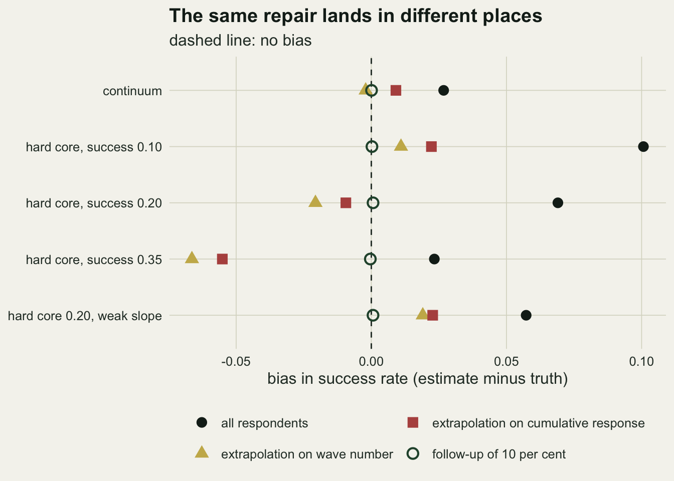
Three hard cores the returned forms cannot tell apart
The three hard core populations that differ only in their hard core’s success were built from the same random draws, and each survey index uses the same seed in all three. So the three offices receive the same forms, from the same hunters, stamped with the same waves.
twin_cols <- c("first", "allresp", "last", "ext_wave", "ext_cum", "rr")
twin_gap <- max(abs(sims[[2]][, twin_cols] - sims[[3]][, twin_cols]),
                abs(sims[[3]][, twin_cols] - sims[[4]][, twin_cols]))
twin_est <- mean(sims[[3]][, "ext_cum"])
twin_truth <- truth[2:4]
The largest difference between the three populations in any quantity computed from the returned forms, in any of the 1000 surveys, is 0: every survey gives the same first wave mean, the same all respondent mean and the same extrapolation in all three, averaging 0.291 on cumulative response, while the true success rates are 0.269, 0.300 and 0.346. The share of bias removed by that single number ranges from 78 to 336 per cent depending on a quantity that never reaches the office.
That construction is deliberately blunt, since a hard core by definition leaves no forms. The sharper question is how wide the ignorance is for a given pile of forms. Suppose each hunter has a fixed chance of answering each mailing. Then the expected number of successful hunters answering wave one, two and three depends on that chance only through its first three moments among the successful hunters, and the same holds for the unsuccessful. Hunters whose chance is zero, or close enough to zero, leave no trace in those moments. The smallest number of successful hunters consistent with the forms is therefore a moment problem, and its answer puts all of them in two response classes, one that always answers the first mailing and one that answers with a single fixed chance. Everyone else in the frame could be a successful or an unsuccessful non-respondent in any proportion. That gives the range of population success rates the forms allow, in closed form.
min_mass <- function(m) {                  # m: first three raw moments times class share
  q <- (m[2] - m[3]) / (m[1] - m[2])
  b <- (m[1] - m[2]) / (1 - q)
  (m[1] - b) + b / q
}
class_moments <- function(P, cls) sapply(1:3, function(k) mean((P$y == cls) * P$p^k))
bound_tab <- t(vapply(pops, function(P)
  c(low = min_mass(class_moments(P, 1)), high = 1 - min_mass(class_moments(P, 0))),
  numeric(2)))
# check the closed form against random three class populations with the same moments
set.seed(3319)
m_chk <- class_moments(pops[[3]], 1)
rand_mass <- replicate(20000, {
  pr <- sort(runif(3)); w <- solve(rbind(pr, pr^2, pr^3), m_chk)
  if (all(w >= 0)) sum(w) else NA
})
n_valid <- sum(!is.na(rand_mass))
mass_gap <- min(rand_mass, na.rm = TRUE) - min_mass(m_chk)
# the same range from one survey's counts: forms by wave, per outcome
forms_moments <- function(cw, n) {        # cw: forms in waves 1 to 3 of one outcome
  m1 <- cw[1] / n; m2 <- m1 - cw[2] / n; c(m1, m2, cw[3] / n - m1 + 2 * m2)
}
plugin_bound <- function(ys, yn, n) {      # NA when noise leaves no valid two class fit
  ms <- forms_moments(ys, n); mf <- forms_moments(yn, n)
  q <- c((ms[2] - ms[3]) / (ms[1] - ms[2]), (mf[2] - mf[3]) / (mf[1] - mf[2]))
  lo <- min_mass(ms); hi <- 1 - min_mass(mf)
  if (all(is.finite(q) & q > 0 & q < 1) && lo >= 0 && hi <= 1 && lo <= hi) c(lo, hi) else c(NA, NA)
}
For the continuum frame, the forms allow any population success rate from 0.336 to 0.390. For the three twin frames the range is the same, as it has to be, and it runs from 0.234 to 0.572. The closed form was checked against 3289 random populations built from three response classes that reproduce the same moments: none needed fewer successful hunters, and the smallest came within 0.00002 of the bound. The continuum range is narrow because only 12 per cent of its licence holders never answer; the hard core range is wide because 38 per cent do. In both cases the range is a statement about the forms, with no assumption about how the non-respondents differ beyond the fixed response chance per mailing, and every extrapolation is one guess inside it.
wave_curve <- function(P, lab) {
  g <- sapply(1:3, function(w) P$p * (1 - P$p)^(w - 1))
  cnt <- colMeans(g); succ <- colSums(P$y * g) / colSums(g)
  cum <- cumsum(cnt); mid <- (c(0, cum[1:2]) + cum) / 2
  nr_mid <- (cum[3] + 1) / 2
  ext <- clamp01(wls_pred(matrix(mid), matrix(succ), matrix(cnt), nr_mid))
  nr_true <- sum(P$y * (1 - P$p)^3) / sum((1 - P$p)^3)
  ar <- sum(succ * cnt) / cum[3]
  list(line = data.frame(panel = lab, x = mid, succ = succ),
       ext = data.frame(panel = lab, x = c(max(mid), nr_mid), succ = c(succ[3], ext)),
       nr_true = nr_true, nr_mid = nr_mid, ext_val = ext,
       nr_low = (bound_tab_lookup(P)[1] - cum[3] * ar) / (1 - cum[3]),
       nr_high = (bound_tab_lookup(P)[2] - cum[3] * ar) / (1 - cum[3]))
}
bound_tab_lookup <- function(P)
  c(min_mass(class_moments(P, 1)), 1 - min_mass(class_moments(P, 0)))
panel_lev <- c("continuum", "three hard cores, one set of forms")
wc_c <- wave_curve(pops[[1]], panel_lev[1])
wc_h <- lapply(2:4, function(i) wave_curve(pops[[i]], panel_lev[2]))
lines_df <- rbind(wc_c$line, wc_h[[1]]$line)
ext_df <- rbind(wc_c$ext, wc_h[[1]]$ext)
lines_df$panel <- factor(lines_df$panel, levels = panel_lev)
ext_df$panel <- factor(ext_df$panel, levels = panel_lev)
truth_df <- data.frame(panel = factor(c(panel_lev[1], rep(panel_lev[2], 3)), levels = panel_lev),
                       x = c(wc_c$nr_mid, rep(wc_h[[1]]$nr_mid, 3)),
                       succ = c(wc_c$nr_true, vapply(wc_h, function(w) w$nr_true, 0)),
                       lab = c("true", "0.10", "0.20", "0.35"))
range_df <- data.frame(panel = factor(panel_lev, levels = panel_lev),
                       x = c(wc_c$nr_mid, wc_h[[1]]$nr_mid) - 0.035,
                       lo = clamp01(c(wc_c$nr_low, wc_h[[1]]$nr_low)),
                       hi = clamp01(c(wc_c$nr_high, wc_h[[1]]$nr_high)))
extp_df <- data.frame(panel = factor(panel_lev, levels = panel_lev),
                      x = c(wc_c$nr_mid, wc_h[[1]]$nr_mid),
                      succ = c(wc_c$ext_val, wc_h[[1]]$ext_val))
fig_waves <- ggplot() +
  geom_errorbar(data = range_df, aes(x = x, ymin = lo, ymax = hi), width = 0.015,
                colour = te_gold, linewidth = 0.9) +
  geom_line(data = ext_df, aes(x, succ), colour = te_rust, linetype = "dashed", linewidth = 0.8) +
  geom_line(data = lines_df, aes(x, succ), colour = te_ink, linewidth = 1) +
  geom_point(data = lines_df, aes(x, succ), colour = te_ink, size = 2.6) +
  geom_point(data = extp_df, aes(x, succ), shape = 21, fill = te_paper, colour = te_rust,
             size = 3.4, stroke = 1.2) +
  geom_point(data = truth_df, aes(x, succ), colour = te_forest, shape = 18, size = 3.8) +
  geom_text(data = truth_df, aes(x, succ, label = lab), colour = te_forest, hjust = -0.3,
            size = 3.3) +
  facet_wrap(~ panel) +
  scale_x_continuous(limits = c(0, 1.12), breaks = seq(0, 1, 0.25)) +
  scale_y_continuous(limits = c(0, 1)) +
  labs(x = "cumulative response rate (wave midpoints)", y = "success rate",
       title = "The forms fix the curve, not the non-respondents",
       subtitle = "black: waves; open red: extrapolated; green: truth, by hard core success;\ngold: non-respondent success the forms allow") +
  theme_datasheet() +
  theme(strip.text = element_text(colour = te_ink, face = "bold"))
fig_waves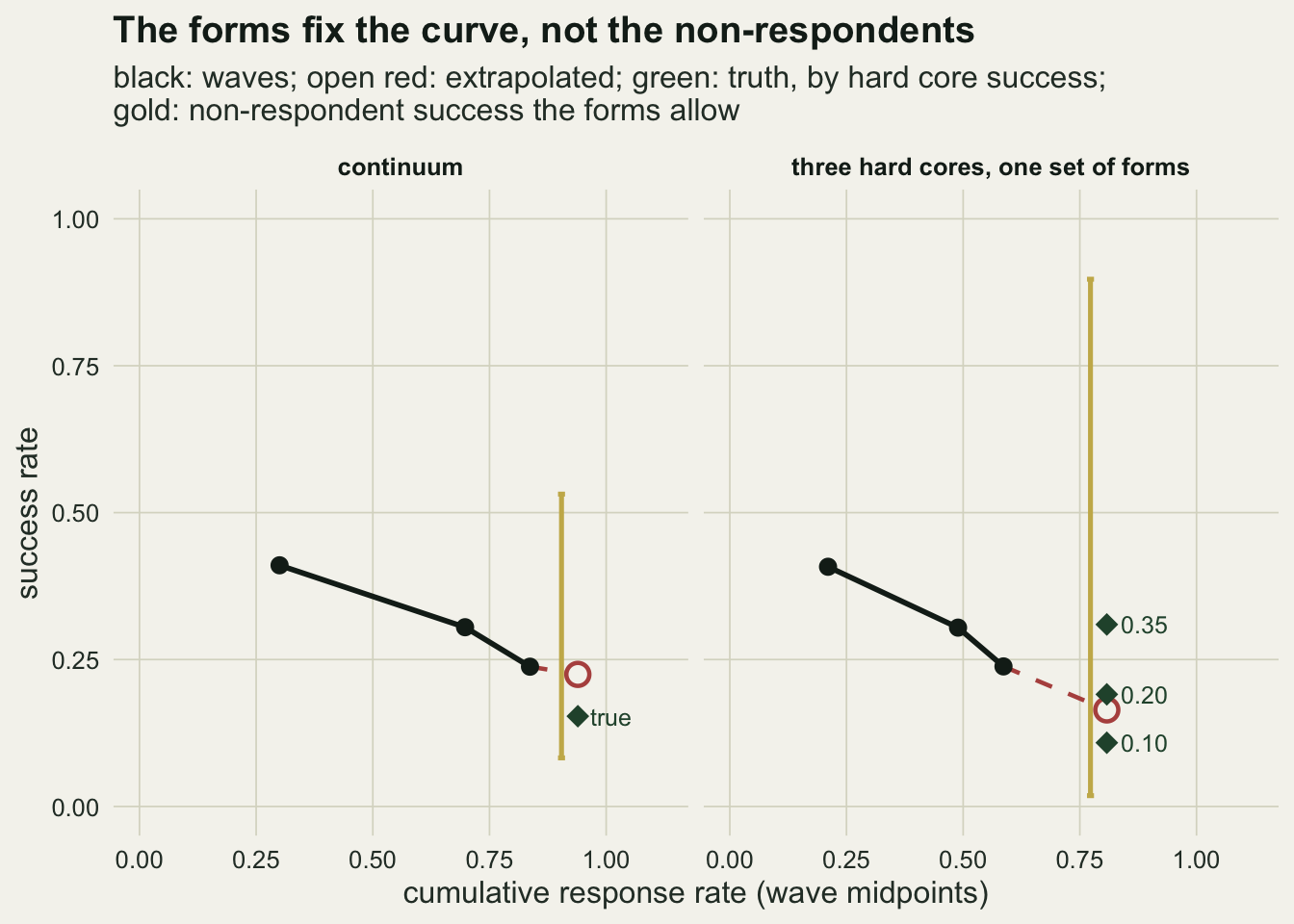
Going back to a random subsample
The follow-up has no such problem, because it does not predict the non-respondents from the respondents. It measures them. Its conditions are that the subsample is random and that the subsampled licence holders who are reached are a random part of it. Three contact regimes test the second condition: contact of 0.7 for everyone, contact of 0.4 for everyone, which is closer to current telephone contact rates, and contact of 0.8 for successful hunters against 0.6 for unsuccessful ones, since a hunter with a deer is happier to talk about it.
hh_summary <- function(cs, k) t(vapply(seq_along(pops), function(i) {
  e <- sims[[i]][, paste0("hh_", cs, "_", k)]; v <- sims[[i]][, paste0("hv_", cs, "_", k)]
  ok <- is.finite(v)
  c(bias = mean(e[ok]) - truth[i], rmse = sqrt(mean((e[ok] - truth[i])^2)),
    cover = mean(abs(e[ok] - truth[i]) <= qnorm(0.975) * sqrt(v[ok])),
    failed = mean(!ok), reached = mean(sims[[i]][, paste0("hm_", cs, "_", k)]))
}, numeric(5)))
fu <- lapply(names(contact_sets), function(cs) lapply(sub_fracs, function(k) hh_summary(cs, k)))
names(fu) <- names(contact_sets)
cover_ext <- vapply(seq_along(pops), function(i)
  mean(sims[[i]][, "ext_lo"] <= truth[i] & sims[[i]][, "ext_hi"] >= truth[i]), 0)
mcse_cover <- sqrt(0.05 * 0.95 / n_rep)
dep_bias <- fu$dependent[[2]][, "bias"]
dep_ratio <- dep_bias / bias_tab["allresp", ]
With independent contact of 0.7 and a ten per cent subsample, the follow-up reaches about 81 non-respondents per survey in the hard core populations, and its nominal 95 per cent interval covers the truth in all five frames between 93.2 and 93.9 per cent of the time, with a Monte Carlo standard error of 0.7 points: slightly short of nominal, since the non-respondent mean is a binary mean from a subsample of that size. At a five per cent subsample the coverage drops to between 90.0 and 93.4 per cent, because the non-respondent mean then rests on a few dozen binary answers or fewer and the normal interval is too short. Cutting contact to 0.4 keeps the bias between -0.0002 and +0.0005 and raises the root mean square error at the ten per cent subsample from between 0.0114 and 0.0211 to between 0.0141 and 0.0281. Low contact that is random costs no bias, but it costs precision and, with a small subsample, interval coverage: at contact 0.4 the interval covers between 90.5 and 94.1 per cent at a ten per cent subsample and between 78.2 and 92.9 per cent at five per cent, where the continuum reaches only 7 non-respondents per survey on average.
Contact that depends on success is different. The follow-up then oversamples successful non-respondents and its bias becomes 0.0052 in the continuum and between 0.0123 and 0.0242 in the hard core frames. The non-respondent share is 0.12 in the continuum, 0.38 in each of the three twin frames and 0.40 in the weak slope frame, so the bias is larger where the non-respondent group is larger only in the contrast of continuum against hard core. Among the twins, at the same group size, it grows with the hard core’s own success (0.0123, 0.0191 and 0.0242), because the contact gap then shifts more of the reached non-respondents towards a harvest; the weak slope frame has the largest share and less bias than the 0.35 twin. Coverage at the ten per cent subsample is 94.7 per cent in the continuum, where few are followed up, and falls to between 82.6 and 90.2 per cent in the hard core frames. A larger subsample makes it worse, not better: at twenty per cent the hard core frames cover between 68.2 and 86.2 per cent, because the bias stays while the interval shrinks. The follow-up has moved the non-response problem one step down, into the subsampled hunters it failed to reach. How much that leaves depends on the frame: the remaining bias is 12 per cent of the all respondent bias in the hard core frame whose non-respondents hunt least, and 104 per cent in the one whose hard core hunts as well as everyone else, where the respondents were only mildly biased to begin with.
The bootstrap interval for extrapolation on cumulative response covers the truth 85.1 per cent of the time in the continuum and 73.5, 90.6, 13.3 and 75.5 per cent in the hard core frames. The bootstrap resamples the forms, so it measures the sampling noise of the extrapolation and nothing about whether the straight line was the right model for the non-respondents; its coverage tracks the bias, not the design.
cov_df <- data.frame(
  population = factor(rep(pop_lev, 4), levels = rev(pop_lev)),
  method = factor(rep(c("extrapolation, bootstrap", "follow-up, contact 0.7",
                        "follow-up, contact 0.4", "follow-up, contact by success"),
                      each = length(pop_lev)),
                  levels = c("extrapolation, bootstrap", "follow-up, contact 0.7",
                             "follow-up, contact 0.4", "follow-up, contact by success")),
  cover = c(cover_ext, fu$independent[[2]][, "cover"], fu$low[[2]][, "cover"],
            fu$dependent[[2]][, "cover"]))
ggplot(cov_df, aes(cover, population, colour = method, shape = method)) +
  geom_vline(xintercept = 0.95, colour = te_body, linetype = "dashed", linewidth = 0.5) +
  geom_point(size = 3, stroke = 1.1, position = position_dodge(width = 0.55)) +
  scale_colour_manual(values = c(te_rust, te_forest, te_gold, te_ink), name = NULL) +
  scale_shape_manual(values = c(15, 16, 17, 4), name = NULL) +
  scale_x_continuous(limits = c(0, 1), breaks = seq(0, 1, 0.2)) +
  guides(colour = guide_legend(nrow = 2)) +
  labs(x = "coverage of the nominal 95 per cent interval", y = NULL,
       title = "Extrapolation intervals miss; random follow-up stays close",
       subtitle = "dashed line: 95 per cent") +
  theme_datasheet() + theme(legend.position = "bottom", plot.title.position = "plot")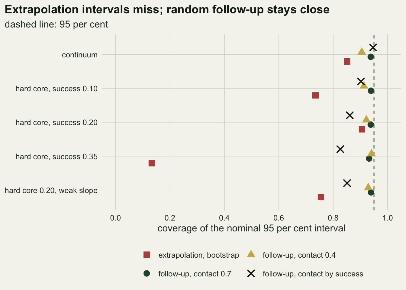
The same budget spent two ways
A follow-up is not free, and the fair comparison holds the money fixed. The costs below are assumptions fixed before running: one unit per form mailed and eight units per subsampled non-respondent, which covers repeated call attempts and the interview. The budget is what a three thousand licence survey with three mailings and a ten per cent follow-up would cost in each frame. Two ways of spending it without a telephone are tried: a larger sample with three mailings, and a fourth mailing, which buys a smaller sample but raises the response rate and shortens the extrapolation. Spending it on a five or twenty per cent follow-up buys a sample larger or smaller than three thousand.
c_mail   <- 1     # cost per form mailed
c_follow <- 8     # cost per subsampled non-respondent
n_cost   <- 500   # surveys per cell in this section
budget_n <- function(P, k, budget) {
  per_unit <- mean(1 + (1 - P$p) + (1 - P$p)^2) * c_mail + mean((1 - P$p)^3) * k * c_follow
  floor(budget / per_unit)
}
k_grid <- c(0, sub_fracs)
cost_tab <- do.call(rbind, lapply(seq_along(pops), function(i) {
  P <- pops[[i]]
  budget <- n_samp * (mean(1 + (1 - P$p) + (1 - P$p)^2) * c_mail +
                      mean((1 - P$p)^3) * 0.10 * c_follow)
  n4 <- floor(budget / (mean(1 + (1 - P$p) + (1 - P$p)^2 + (1 - P$p)^3) * c_mail))
  r4 <- run_pop(P, seed0 = 96000, n = n4, boot = FALSE, reps = n_cost, n_mail = 4)
  mail4 <- data.frame(population = pop_lev[i], k = 0, n = n4,
                      method = c("all respondents, four mailings",
                                 "extrapolation, four mailings"),
                      rmse = c(sqrt(mean((r4[, "allresp"] - truth[i])^2)),
                               sqrt(mean((r4[, "ext_cum"] - truth[i])^2))),
                      bias = c(mean(r4[, "allresp"]) - truth[i], mean(r4[, "ext_cum"]) - truth[i]),
                      rr = mean(r4[, "rr"]))
  rbind(mail4, do.call(rbind, lapply(seq_along(k_grid), function(j) {
    k <- k_grid[j]; nk <- budget_n(P, k, budget)
    r <- run_pop(P, seed0 = 90000 + 1000 * j, n = nk, boot = FALSE, reps = n_cost)
    if (k == 0) {
      data.frame(population = pop_lev[i], k = k, n = nk,
                 method = c("all respondents", "extrapolation on cumulative response"),
                 rmse = c(sqrt(mean((r[, "allresp"] - truth[i])^2)),
                          sqrt(mean((r[, "ext_cum"] - truth[i])^2))),
                 bias = c(mean(r[, "allresp"]) - truth[i], mean(r[, "ext_cum"]) - truth[i]),
                 rr = mean(r[, "rr"]))
    } else {
      e <- r[, paste0("hh_independent_", k)]
      data.frame(population = pop_lev[i], k = k, n = nk, method = "follow-up",
                 rmse = sqrt(mean((e - truth[i])^2, na.rm = TRUE)),
                 bias = mean(e, na.rm = TRUE) - truth[i], rr = mean(r[, "rr"]))
    }
  })))
}))
cost_tab$population <- factor(cost_tab$population, levels = pop_lev)
ct_col <- function(pop, meth, k, col) cost_tab[[col]][cost_tab$population == pop &
                                                   cost_tab$method == meth & cost_tab$k == k]
ct <- function(pop, meth, k) ct_col(pop, meth, k, "rmse")
fu_sub <- cost_tab[cost_tab$method == "follow-up", ]
fu_best <- vapply(pop_lev, function(pp) min(fu_sub$rmse[fu_sub$population == pp]), 0)
fu_best_k <- vapply(pop_lev, function(pp) fu_sub$k[fu_sub$population == pp][which.min(fu_sub$rmse[fu_sub$population == pp])], 0)
ext0 <- vapply(pop_lev, function(pp) ct(pp, "extrapolation on cumulative response", 0), 0)
n0 <- vapply(pop_lev, function(pp) ct_col(pp, "all respondents", 0, "n"), 0)
n4 <- vapply(pop_lev, function(pp) ct_col(pp, "extrapolation, four mailings", 0, "n"), 0)
ext4 <- vapply(pop_lev, function(pp) ct(pp, "extrapolation, four mailings", 0), 0)
ext4_bias <- vapply(pop_lev, function(pp) ct_col(pp, "extrapolation, four mailings", 0, "bias"), 0)
ext3_bias <- vapply(pop_lev, function(pp) ct_col(pp, "extrapolation on cumulative response", 0, "bias"), 0)
all4 <- vapply(pop_lev, function(pp) ct(pp, "all respondents, four mailings", 0), 0)
rr3 <- vapply(pop_lev, function(pp) ct_col(pp, "all respondents", 0, "rr"), 0)
rr4 <- vapply(pop_lev, function(pp) ct_col(pp, "extrapolation, four mailings", 0, "rr"), 0)
fu5 <- vapply(pop_lev, function(pp) ct(pp, "follow-up", 0.05), 0)
all0 <- vapply(pop_lev, function(pp) ct(pp, "all respondents", 0), 0)
best_plain <- pmin(ext0, all0, ext4, all4)
fu5_wins <- fu5 < best_plain
fu20_wins <- vapply(pop_lev, function(pp) ct(pp, "follow-up", 0.2), 0) < best_plain
bias_share <- bias_tab["ext_cum", ]^2 / rmse_tab["ext_cum", ]^2
n20 <- vapply(pop_lev, function(pp) ct_col(pp, "follow-up", 0.2, "n"), 0)
fu20 <- vapply(pop_lev, function(pp) ct(pp, "follow-up", 0.2), 0)
# rough Monte Carlo error of a difference of two independent RMSEs (se of an RMSE ~ RMSE / sqrt(2 R))
mcse_diff <- sqrt(fu20^2 + best_plain^2) / sqrt(2 * n_cost)
fu20_clear <- best_plain - fu20 > 2 * mcse_diff
cbind(n0, n4, n20, all0, ext0, all4, ext4, fu5, fu_best, rr3, rr4, ext3_bias, ext4_bias)
n0 n4 n20 all0 ext0 all4
continuum 3181 2957 2837 0.02763540 0.01257238 0.02011898
hard core, success 0.10 3456 2904 2650 0.10079354 0.02705043 0.09252000
hard core, success 0.20 3456 2904 2650 0.06937131 0.01950210 0.06115954
hard core, success 0.35 3456 2904 2650 0.02503403 0.05837674 0.01778989
hard core 0.20, weak slope 3460 2903 2647 0.05778829 0.02742888 0.05368032
ext4 fu5 fu_best rr3 rr4
continuum 0.01058228 0.01400205 0.01052161 0.8790613 0.9215698
hard core, success 0.10 0.02071257 0.01818069 0.01242947 0.6162934 0.6457300
hard core, success 0.20 0.02271588 0.02289333 0.01488312 0.6162934 0.6457300
hard core, success 0.35 0.06462606 0.02736505 0.01726888 0.6162934 0.6457300
hard core 0.20, weak slope 0.02428878 0.02494173 0.01509780 0.6047451 0.6380048
ext3_bias ext4_bias
continuum 0.008698537 0.006195871
hard core, success 0.10 0.021376241 0.014450585
hard core, success 0.20 -0.010273759 -0.017199415
hard core, success 0.35 -0.055973759 -0.062899415
hard core 0.20, weak slope 0.021866030 0.018395538With three mailings and no follow-up the budget buys 3181 licences in the continuum frame and 3456 in the hard core frames; a fourth mailing leaves 2957 and 2904, and a twenty per cent follow-up 2837 and 2650. The fourth mailing lifts the response rate from 87.9 to 92.2 per cent in the continuum, but only from 61.6 to 64.6 per cent in the hard core frames, since the hard core does not answer a fourth letter either.
In the continuum, extrapolation on cumulative response has a root mean square error of 0.0126 with three mailings and 0.0106 with four, against 0.0105 for the best of the three follow-up fractions; the last two differ by less than their rough Monte Carlo error of 0.0005, so here a fourth mailing is as good as a telephone follow-up. In the hard core frames the extrapolation error is 0.0271, 0.0195, 0.0584 and 0.0274 with three mailings and 0.0207, 0.0227, 0.0646 and 0.0243 with four, and the best follow-up reaches 0.0124, 0.0149, 0.0173 and 0.0151, in every frame at the largest fraction tried, 0.20. The fourth mailing moves the extrapolation bias from +0.0214 to +0.0145 in the 0.10 frame and from +0.0219 to +0.0184 in the weak slope frame, where the line under-corrects, but from -0.0103 to -0.0172 and from -0.0560 to -0.0629 in the two frames where it over-corrects: the extra wave helps the pair of frames where the line falls short and hurts the pair where it overshoots.
The smallest follow-up is rarely worth it. At a five per cent subsample it is worse than three mailings with extrapolation in the continuum (0.0140 against 0.0126) and in the 0.20 frame (0.0229 against 0.0195), and in the 0.35 frame it is worse than the plain respondent mean (0.0274 against 0.0250); it beats every mail-only option in 1 of the five frames, while the twenty per cent follow-up is below every mail-only option in 5 of the five, and by more than twice the rough Monte Carlo error in 3. In the frame whose hard core hunts as well as everyone else, the plain all respondent mean at the same budget has an error of 0.0250 with three mailings, less than half the extrapolation error: there the repair is worse than no repair, and with four mailings the plain mean reaches 0.0178, which the best follow-up (0.0173) beats by less than its rough Monte Carlo error of 0.0008: a second frame where mail alone ties the telephone. The follow-up error is variance, which a larger subsample reduces. The extrapolation error is partly bias, which a larger sample does not touch and a fourth mailing only moves: at three thousand licences the bias makes up 52 per cent of its mean squared error in the continuum and between 22 and 91 per cent in the hard core frames, and which end a real survey sits at is again not in the forms.
fu_df <- cost_tab[cost_tab$method == "follow-up", ]
flat_df <- cost_tab[cost_tab$k == 0 & cost_tab$method != "all respondents, four mailings", ]
meth_lev <- c("all respondents", "extrapolation on cumulative response",
              "extrapolation, four mailings", "follow-up")
ggplot() +
  geom_hline(data = flat_df, aes(yintercept = rmse, colour = method, linetype = method),
             linewidth = 0.8) +
  geom_line(data = fu_df, aes(k, rmse, colour = method, linetype = method), linewidth = 0.9) +
  geom_point(data = fu_df, aes(k, rmse, colour = method), size = 2.4) +
  facet_wrap(~ population, nrow = 2) +
  scale_colour_manual(values = c("all respondents" = te_ink,
                                 "extrapolation on cumulative response" = te_rust,
                                 "extrapolation, four mailings" = te_gold,
                                 "follow-up" = te_forest), name = NULL, breaks = meth_lev) +
  scale_linetype_manual(values = c("all respondents" = "dotted",
                                   "extrapolation on cumulative response" = "dashed",
                                   "extrapolation, four mailings" = "longdash",
                                   "follow-up" = "solid"), name = NULL, breaks = meth_lev) +
  scale_x_continuous(breaks = sub_fracs, labels = c("0.05", "0.10", "0.20"),
                     limits = c(0.03, 0.22)) +
  scale_y_continuous(limits = c(0, NA)) +
  guides(colour = guide_legend(ncol = 2), linetype = guide_legend(ncol = 2)) +
  labs(x = "share of non-respondents followed up", y = "root mean square error",
       title = "At equal cost a large follow-up is never beaten",
       subtitle = "each panel one licence frame; lines without points spend the budget on mail") +
  theme_datasheet() +
  theme(legend.position = "bottom", strip.text = element_text(colour = te_ink, size = 9),
        legend.key.width = unit(2.2, "lines"), panel.spacing.x = unit(1.4, "lines"))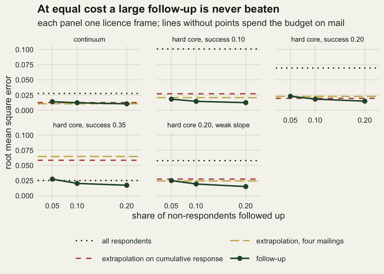
What to report
ex_ys <- tabulate(ex_wave[ex_y == 1], 4)[1:3]; ex_yn <- tabulate(ex_wave[ex_y == 0], 4)[1:3]
ex_bound <- plugin_bound(ex_ys, ex_yn, n_samp)
set.seed(8123)
pb_rep <- t(replicate(200, {              # 200 surveys of the hard core 0.20 frame
  P <- pops[[3]]; s <- sample.int(n_lic, n_samp); p <- P$p[s]; y <- P$y[s]
  u <- matrix(runif(3 * n_samp), n_samp)
  wv <- ifelse(u[, 1] < p, 1L, ifelse(u[, 2] < p, 2L, ifelse(u[, 3] < p, 3L, 4L)))
  plugin_bound(tabulate(wv[y == 1], 4)[1:3], tabulate(wv[y == 0], 4)[1:3], n_samp)
}))
pb_fail <- mean(is.na(pb_rep[, 1]))
pb_excl <- mean(pb_rep[, 1] > truth[3] | pb_rep[, 2] < truth[3], na.rm = TRUE)
pb_q <- apply(pb_rep, 2, quantile, c(0.025, 0.5, 0.975), na.rm = TRUE)
rbind(forms = ex_bound, large_sample = bound_tab[1, ])
low high
forms 0.3408549 0.4154349
large_sample 0.3356410 0.3901475round(pb_q, 3) [,1] [,2]
2.5% 0.223 0.536
50% 0.236 0.571
97.5% 0.252 0.596Report the response rate after each mailing and the success rate of the forms returned in each wave. That table is cheap, every postal survey already has it, and it lets a reader see how steep the respondent gradient is.
If wave extrapolation is used, report it next to the all respondent estimate and say which version was fitted: last wave as a stand-in, a line in wave number, or a line in cumulative response. The versions differ by more than their sampling error in several of the frames here, so the choice is part of the result.
Do not report the bootstrap interval of an extrapolated estimate as if it were a statement about the non-respondents. It describes the forms. The range of success rates the forms allow, under the assumption of a fixed response chance per hunter, is a statement about the non-respondents, and an office can compute it from the wave table: per outcome, the forms returned in waves one to three divided by the sample size give the three moments (the forms_moments() function above), and plugin_bound() turns them into the range. For the worked continuum survey it gives 0.341 to 0.415, against 0.336 to 0.390 from the frame itself. In the hard core frames here, with 38 per cent non-response, the frame range is 0.34 wide on a scale from zero to one. Report it with its sampling spread, as the next section explains.
If the budget allows a random follow-up of non-respondents, it is the only arm here whose bias does not depend on something unobserved. Report the subsample fraction, the number subsampled, the number reached, and the contact rate among the successful and unsuccessful where the reached interviews reveal it. A follow-up with low contact is still unbiased if contact is unrelated to harvest; the report should say why that is believed.
Honest limits
Each hunter’s chance of returning a form is the same for every mailing. Real reminders differ in content and timing, and a stronger final mailing can pull in hunters the first two could not. The closed form range depends on this assumption; with mailing-specific response chances the forms constrain even less. The fourth mailing in the budget section also keeps the same chance, which is kind to it.
The range shown in the figure is the large-sample one, computed from the frame. A single survey’s plug-in varies: over 200 surveys of the hard core 0.20 frame, the middle 95 per cent of plug-in lower ends ran from 0.223 to 0.252 and of upper ends from 0.536 to 0.596, the number of plug-in ranges that missed the true rate of 0.300 was 0, and the number that gave no valid two class fit was 0. The lower ends scatter around the frame value of 0.234; in the continuum survey above, the plug-in upper end sits 0.025 above the frame value, a large move on a range that narrow. A bootstrap of the wave table would put an interval around each end; that is not done here.
Harvest is a single yes or no. Agencies also estimate total harvest and bag size, where a few hunters with many animals dominate the total; the respondent gradient in bag size need not match the gradient in success, and memory errors grow with the delay before the form is filled in, so late respondents may also report less accurately. Neither was simulated.
The hard core populations share one continuum and one hard core size of thirty per cent. That was chosen to make the returned forms identical by construction, and the spread of extrapolation performance it shows is a property of the design, not an estimate of how often real harvest surveys fall at either end.
The follow-up assumes that reached non-respondents answer truthfully and that a telephone interview measures the same thing as the form. Mode effects and recall error are not simulated. The cost ratio of eight to one is an assumption, and the budget comparison moves with it; a short second postal form sent to the subsample is a cheaper instrument whose response may also depend on harvest, which is the dependent contact case above. The design-based interval for the follow-up at a five per cent subsample under-covers because it treats a small binary mean as normal.
The licence type covariate was given no role in response beyond its link to success. A frame covariate that also drives response would give weighting more to work with, as the site substitution post shows.
References
Armstrong JS, Overton TS 1977 Journal of Marketing Research 14(3):396-402 (10.1177/002224377701400320)
Hansen MH, Hurwitz WN 1946 Journal of the American Statistical Association 41(236):517-529 (10.1080/01621459.1946.10501894)
Lin IF, Schaeffer NC 1995 Public Opinion Quarterly 59(2):236 (10.1086/269471)
Groves RM, Peytcheva E 2008 Public Opinion Quarterly 72(2):167-189 (10.1093/poq/nfn011)